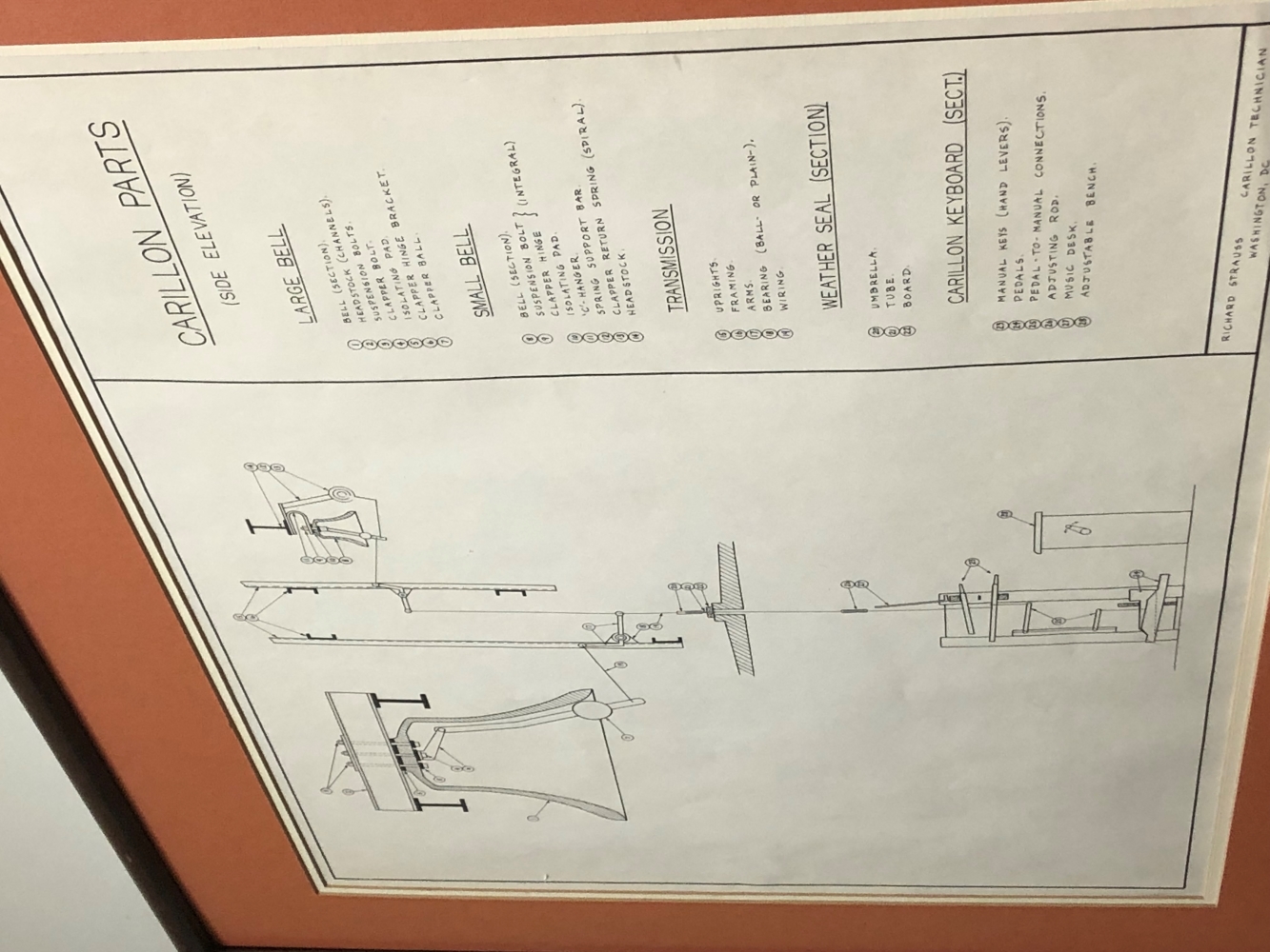
Diagram of the Campanile Bells
In this project, I use homography to rectify images and make basic panoramas.
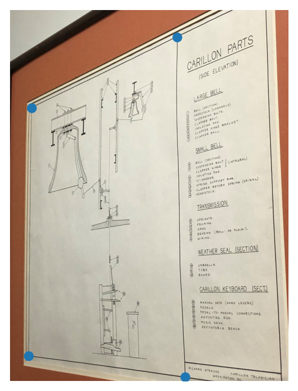
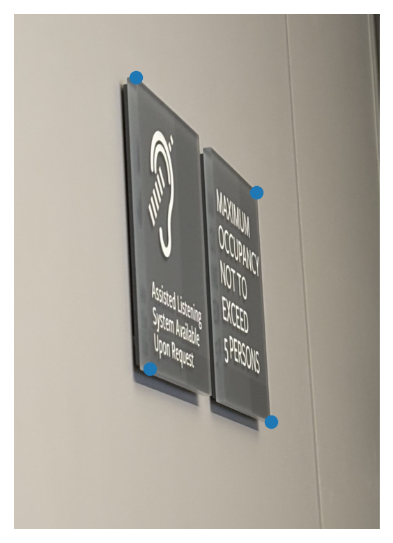
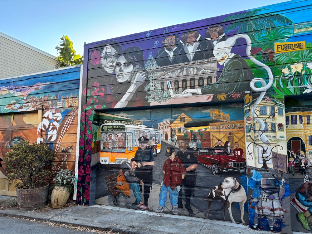
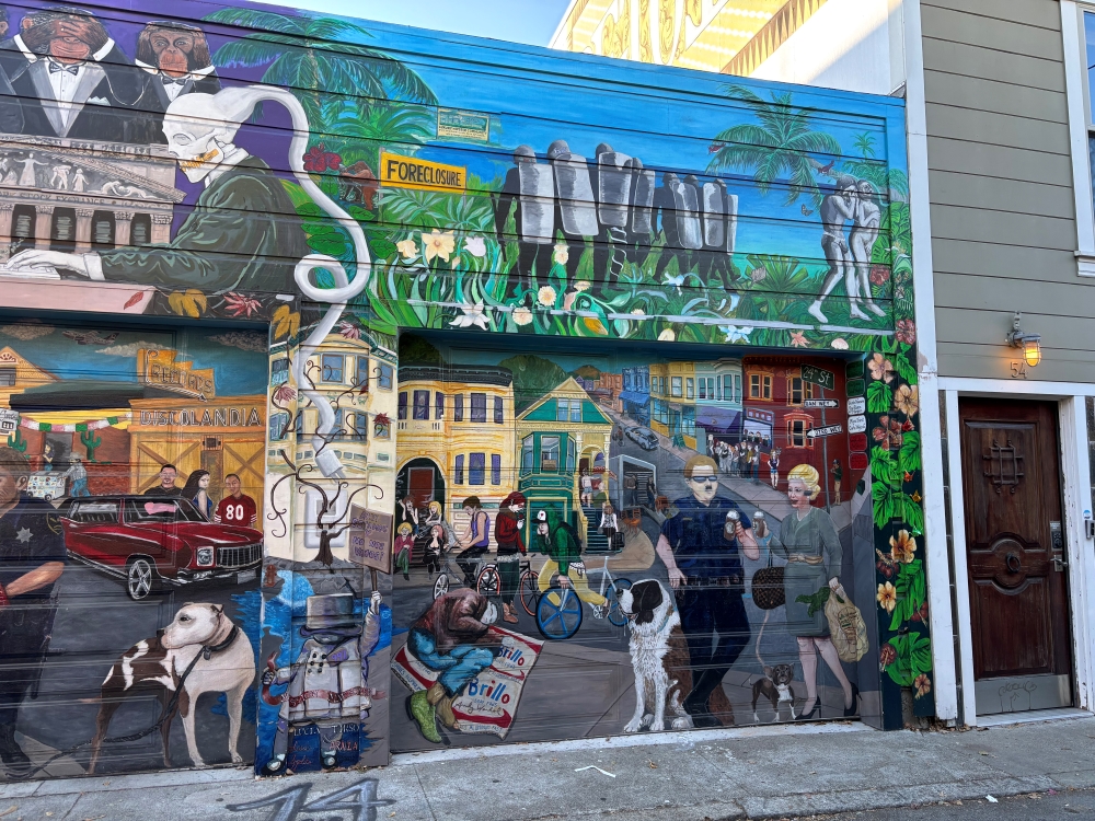
Below are the images I used for the first part of this project (sections 2-4).

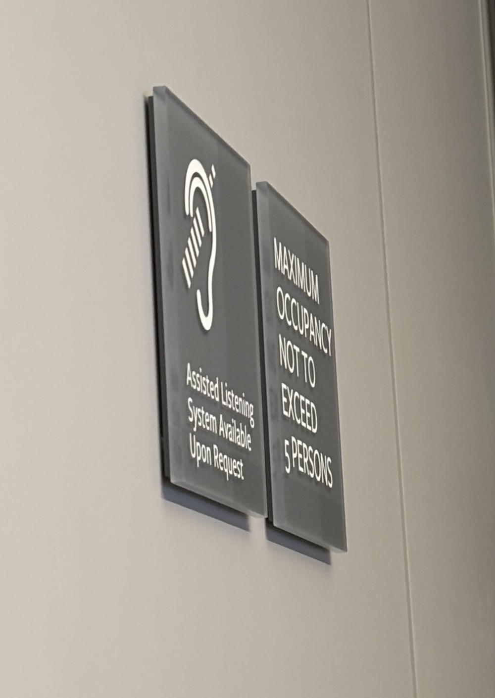
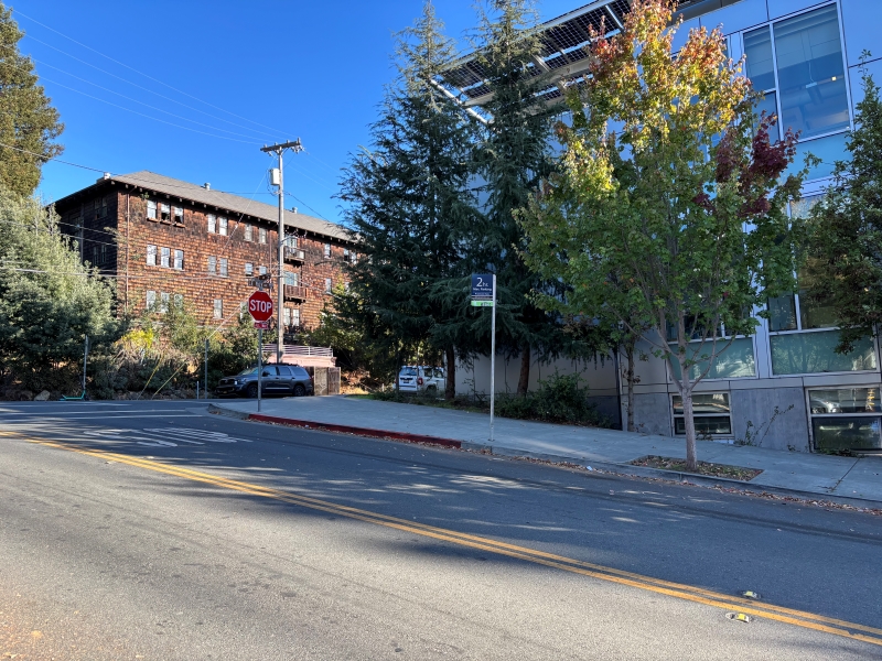
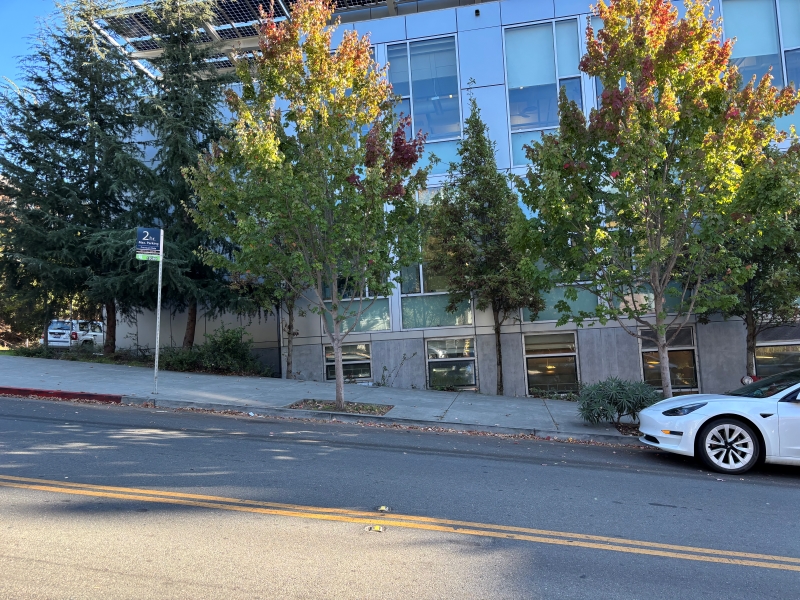
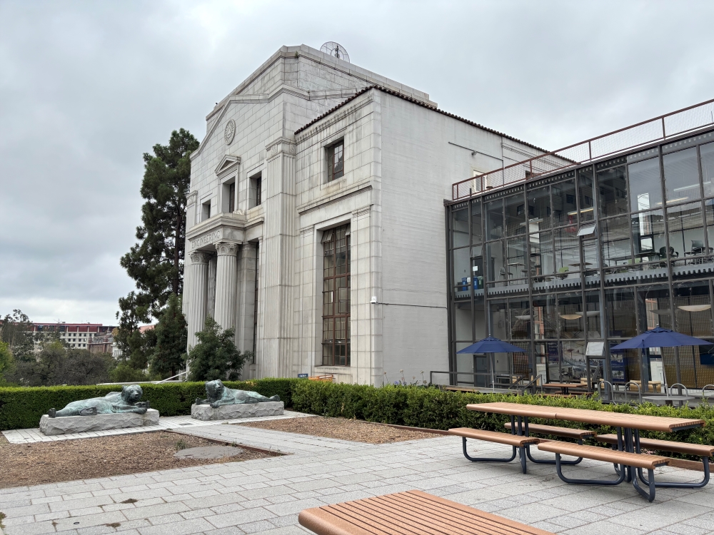
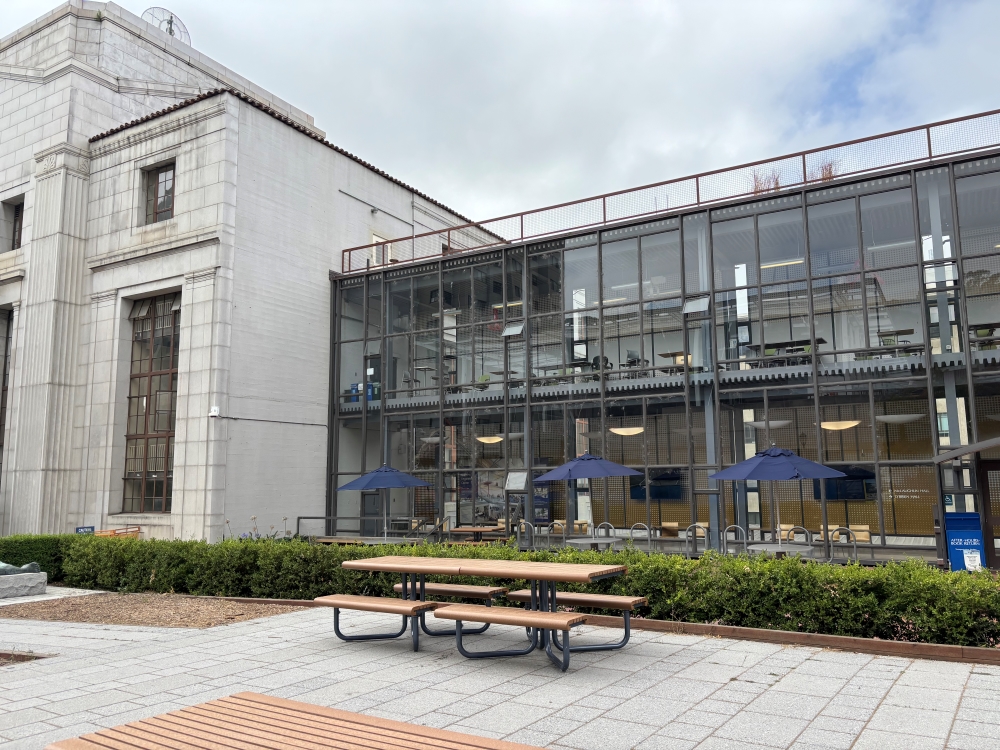
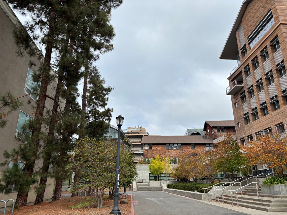
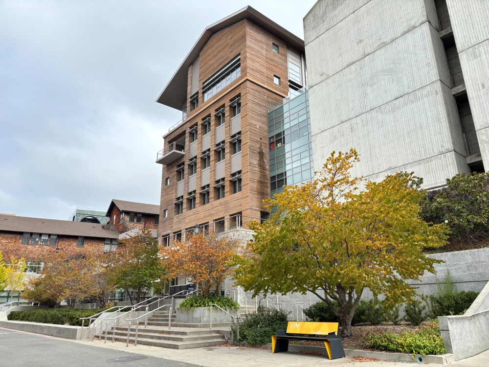
In order to rectify an image or create a panorama, we must compute a homography using correspondence points in order to project an image to the same plane as another image. More specifically, we want to recover a 3x3 matrix such that:

where (x,y) corresponds to a point in our image to reproject, and (x’,y’) corresponds to the reference image whose plane we are aligning the other images to.
To solve for this, we can expand the system out such that the right hand side only consists of our reference image points:
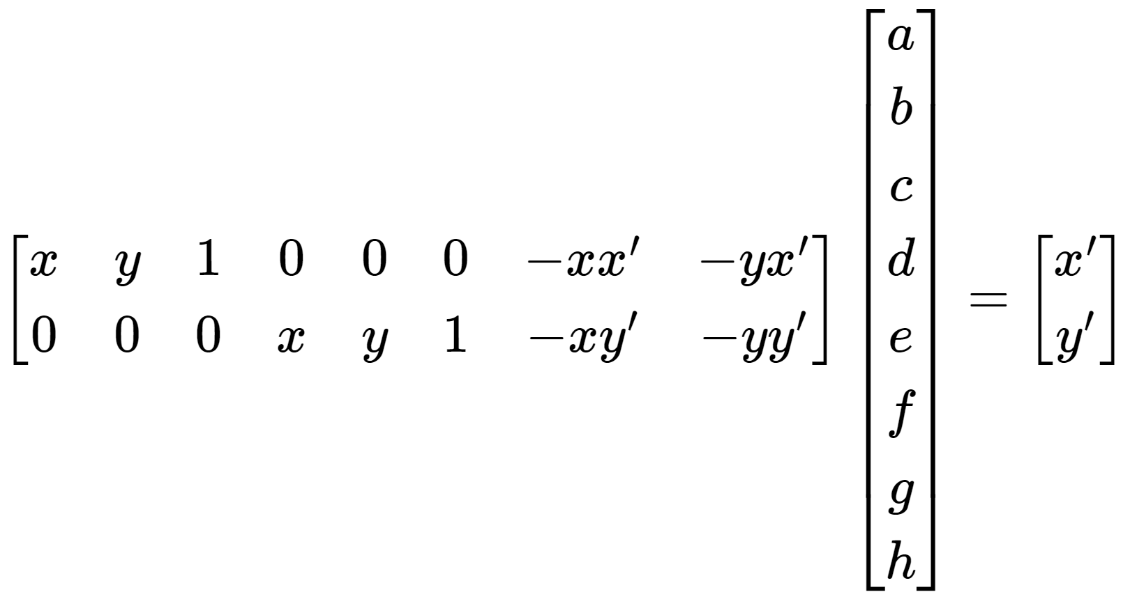
The above equation is only for one point (x,y). When using multiple correspondence points, I used numpy.vstack to stack the points vertically in the corresponding vectors and matrices.
To solve for the homography matrix, I used least-squares, which would account for overdetermined systems.
With the recovered homography matrix h, we can apply the matrix to the corners of an image as a projective transform.
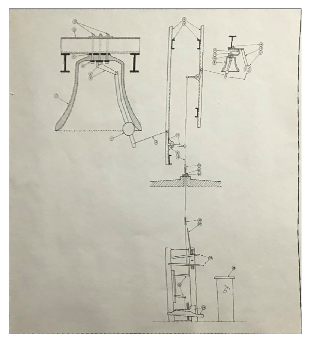
For image rectification, I computed a homography matrix between a rectangle within an image and a manually-defined set of coordinates. Then I transformed the rectangle coordinates within the image using h and divided by the scaling factor w (see the first equation above) to obtain the corresponding warped coordinates. After finding the bounding box of our resulting warp in this way, I used sk.draw.polygon and the inverse of the homography matrix to perform an inverse warp of all the coordinates within the bounding box and extract the corresponding pixel values from the original image.
If the bounding box (after applying h and dividing by w) has negative coordinates, I computed and applied a translation matrix T so that the entire box had positive coordinates. I shifted the coordinates back using the inverse of T to extract the corresponding pixel values.

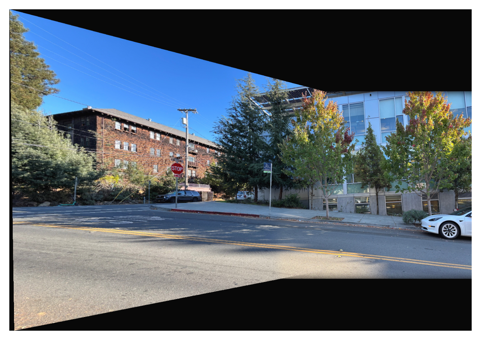
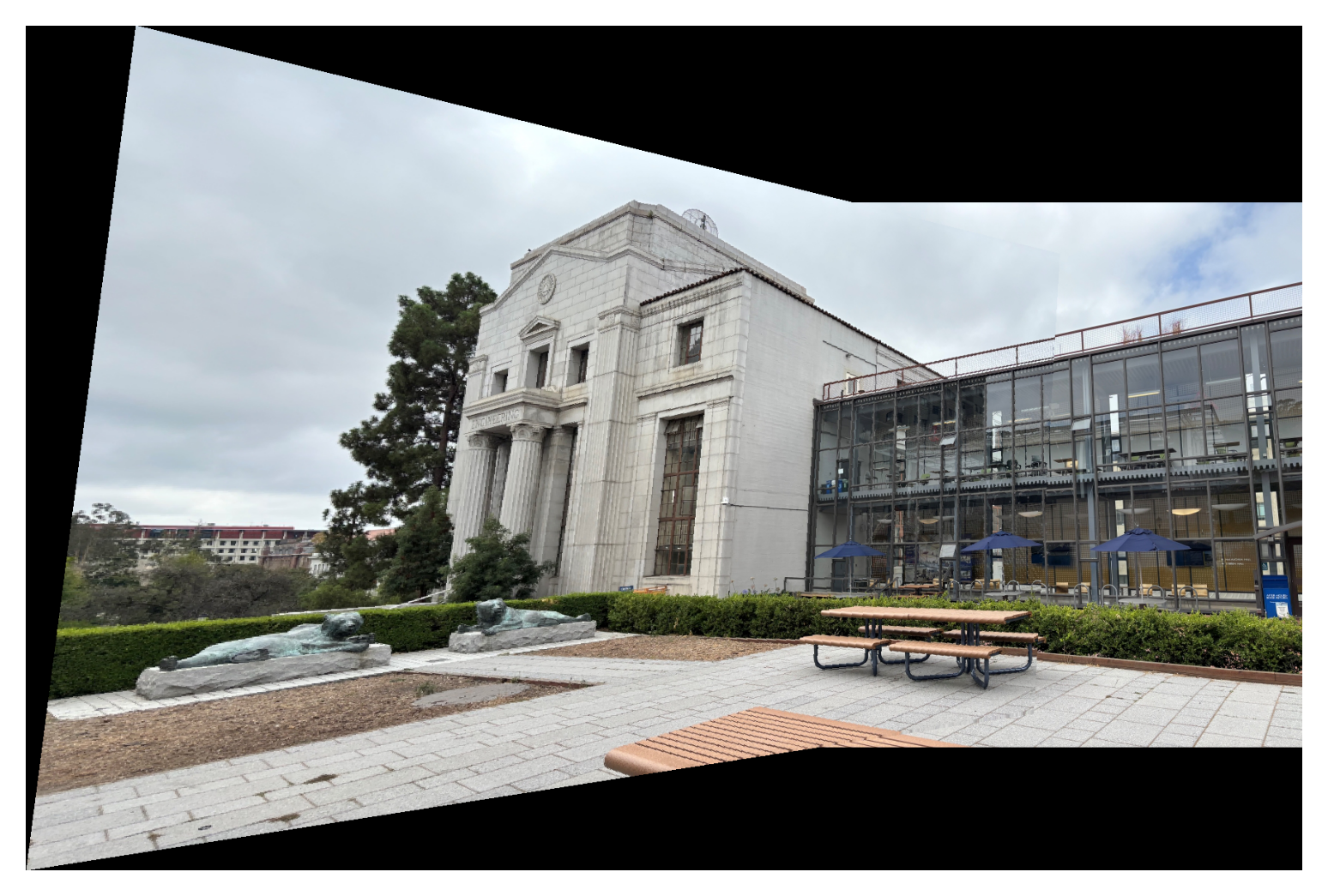
To create a panomara, I can use the same idea as image rectification, but instead of choosing 4 corners, I choose 8 correspondence points to recover my homography matrix.
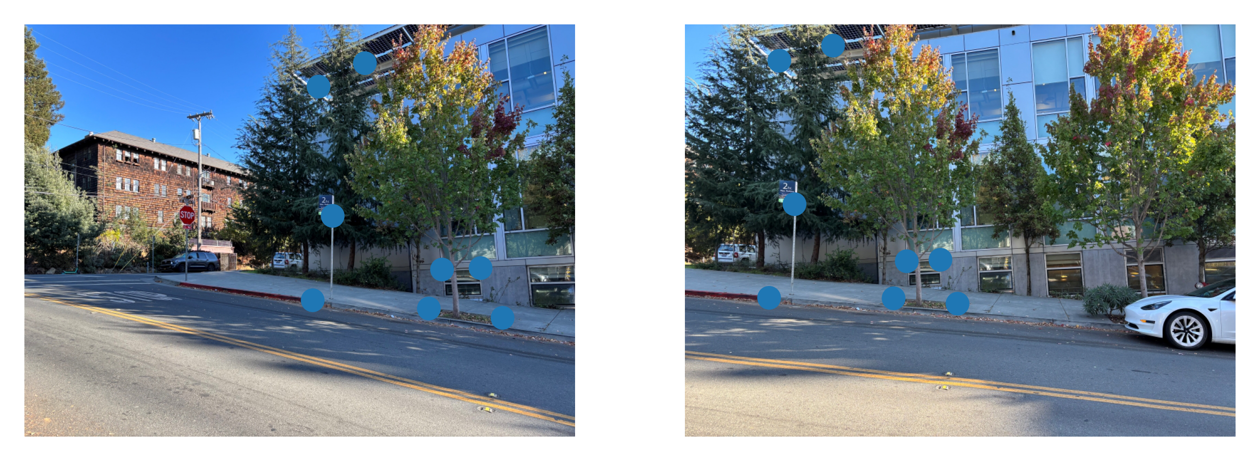
Creating a panorama requires computing a bigger bounding box that encompasses both the warped images and the reference image. To do this, I calculated the bounding boxes of all images after warping and translating (taking into account negative coordinates) and took the max x and y values out of the bounding box coordinates. After computing this bounding box, I created an empty array of the size of the bounding box and populated its elements using pixel values and coordinate indices obtained from the warp and translation tranformations I had saved from prior computations.
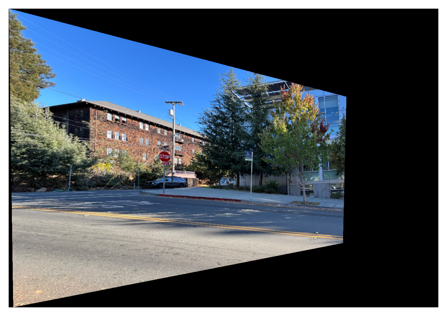
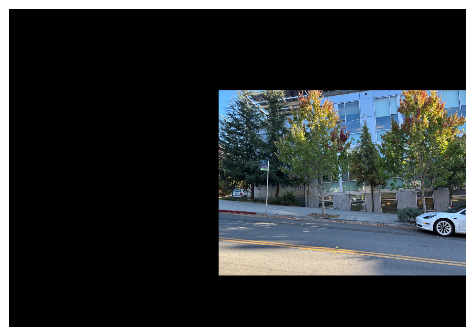
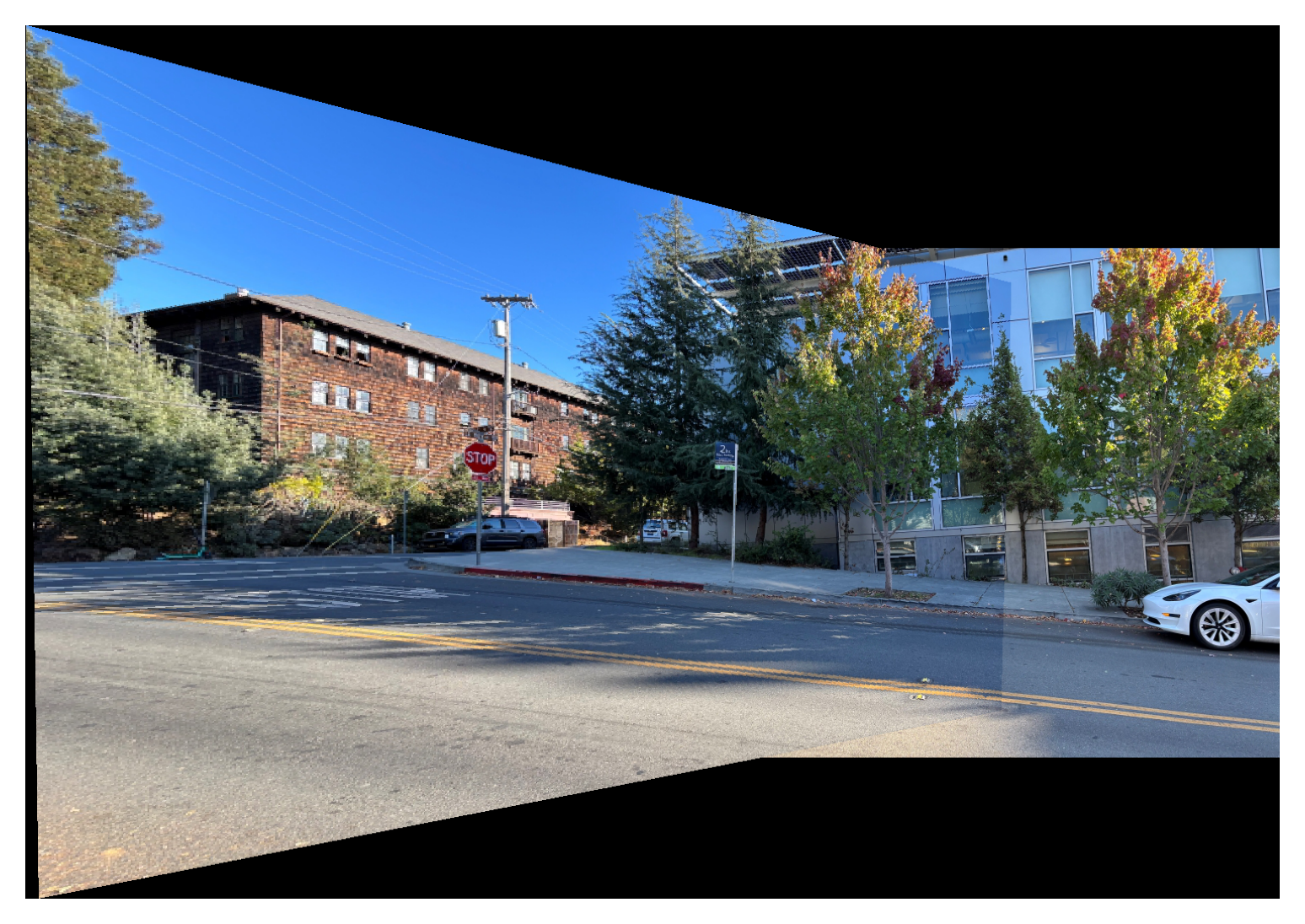
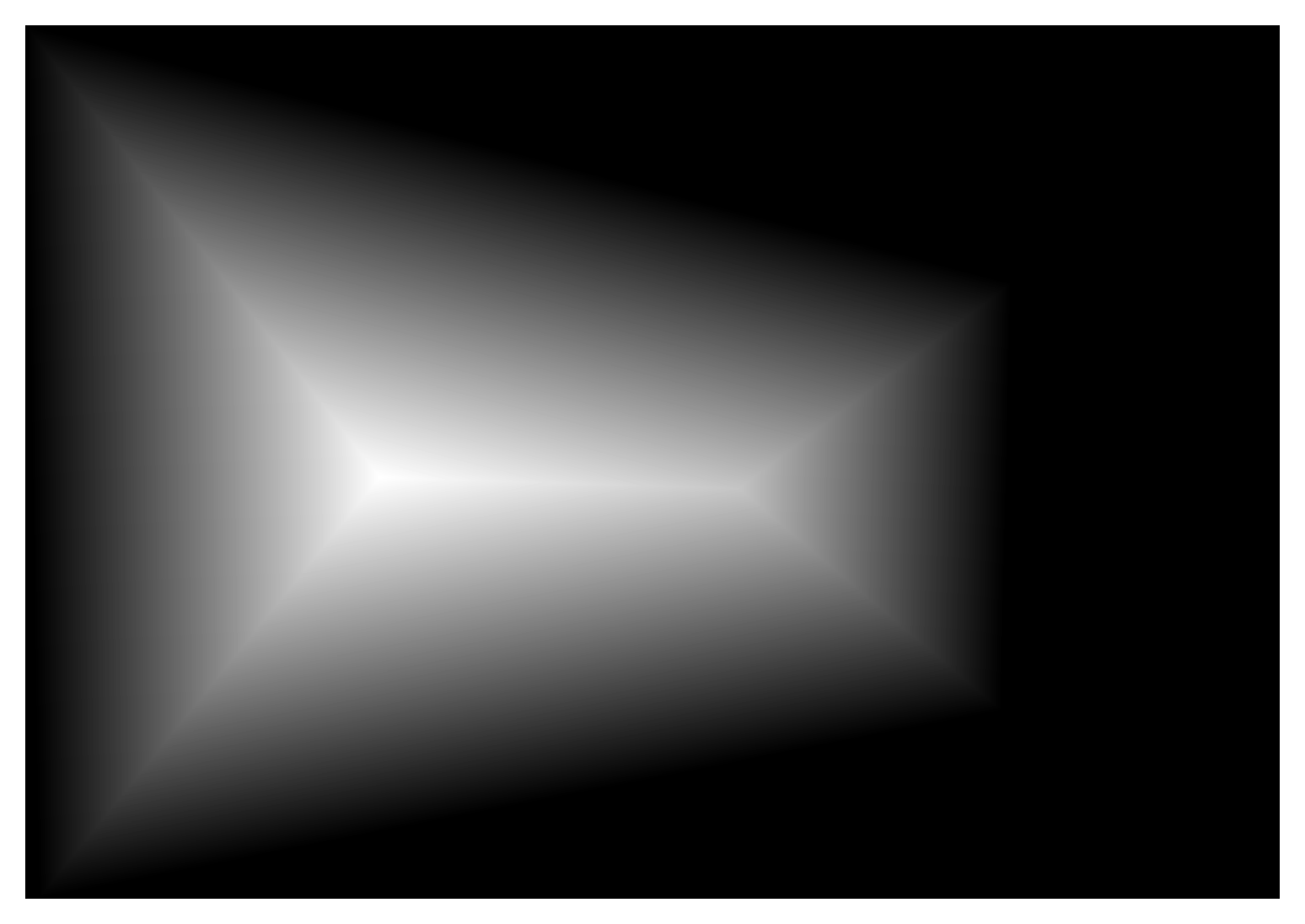
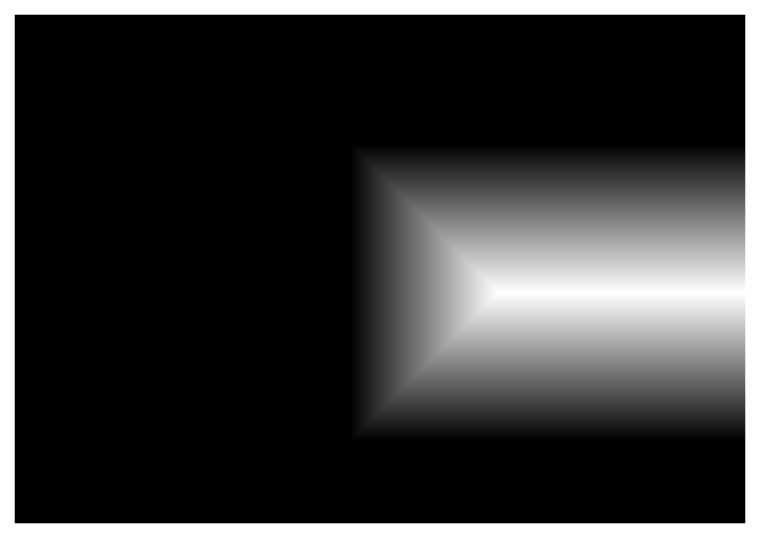
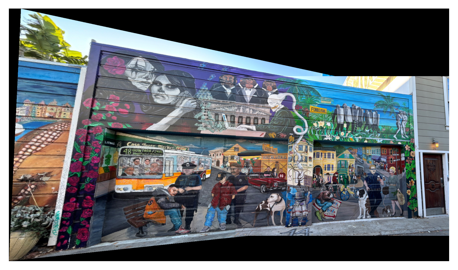
When naively overlaying the warped image onto the reference image, there is often a visible seam due to differences in lighting between the images and human error in selecting the correspondence points. To fix this, I implemented blending. I applied the distance transform between alpha channels and created a mask for the areas where the distance transform value was greater in the warped image.


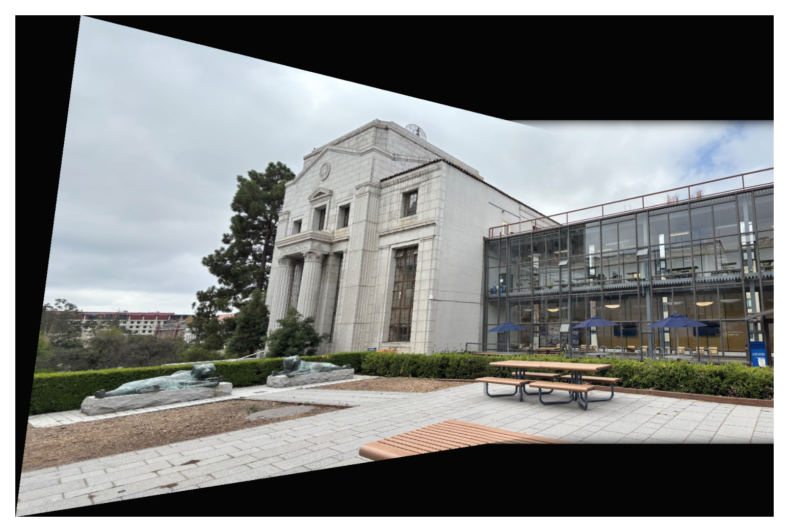
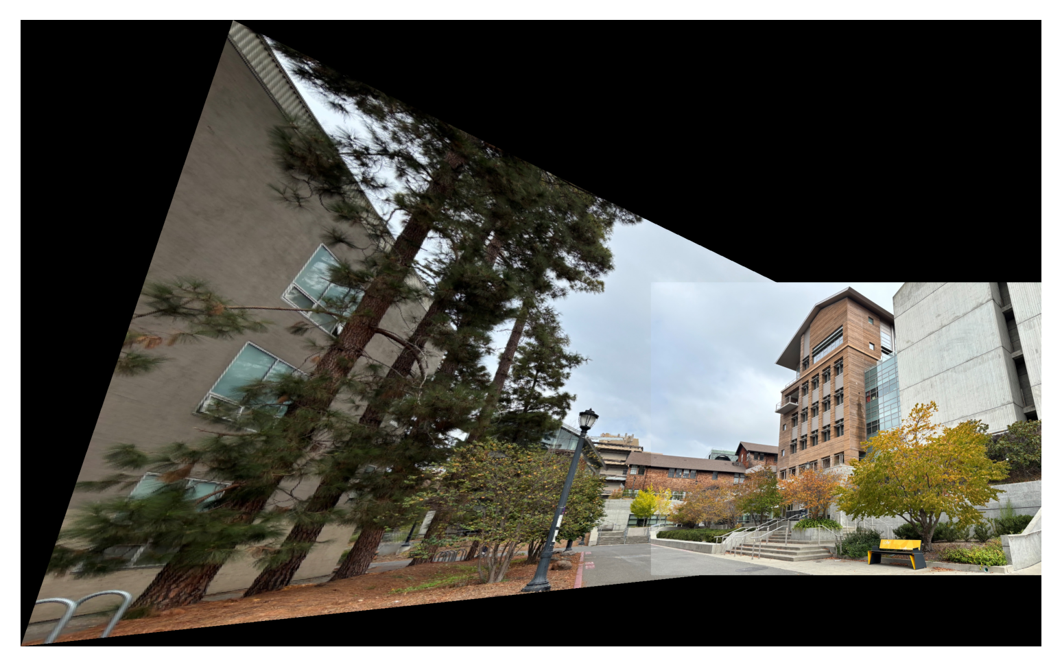
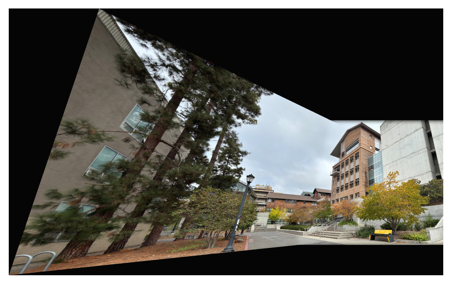
In parts 1-4, I used manually defined correspondence points to compute a homography for the mosaic blending. But manually defining the points for each pair of images can be very tedious and also inaccurate. In the next parts, I implement a pipeline to autodetect suitable correspondence points.
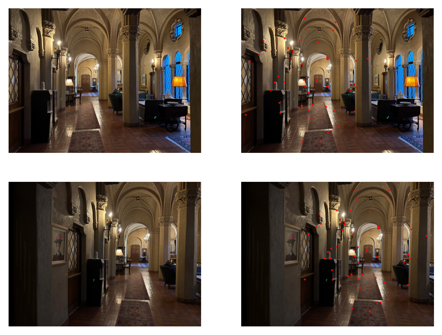
To obtain candidate correspondence points, I use Harris corner detection to detect corners in the two images. Corners are good candidates for correspondence since they capture change in all directions, as opposed to an edge. Corners also worked well when manually defining correspondence points.
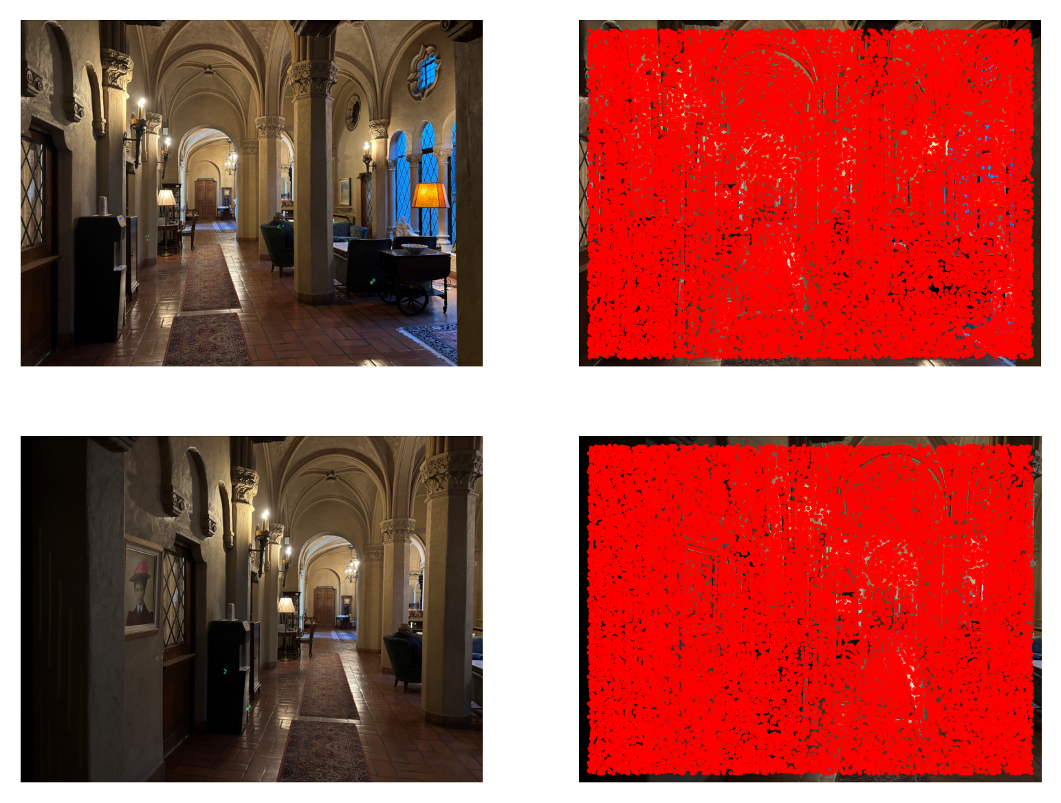
As one might notice above, Harris corner detection picks up too many candidate points… To help filter out candidate points, I implement Adaptive Non-Maximal Supression (ANMS). For each candidate point p, I keep the closest neighbor such that their strength (obtained from the Harris matrix) times the crobust (which I set to 0.9) is greater than the strength of p. I used a KDTree for efficient neighbor searching.
By implementing ANMS, we are able to keep a number of candidate points that are evenly distributed throughout the image AND representing relatively strong corners. We are also able to choose how many candidate points k we would like to keep, by picking the k top points ordered by distance.
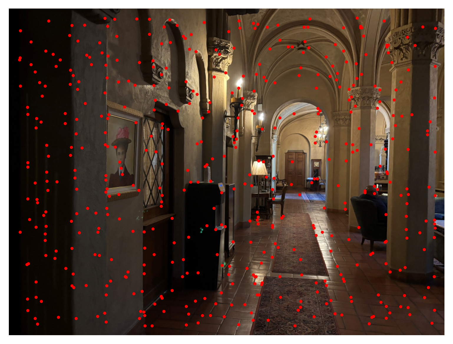
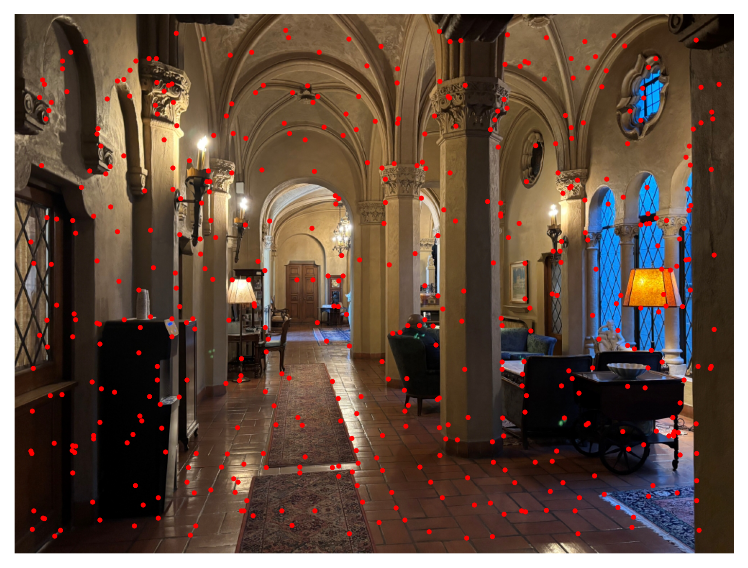
Now that we have our candidate points after ANMS, we would like to further narrow them down by matching them across the two images. First, we extract feature descriptors from each point. This means that for a point p, we obtain the 40x40 pixel patch around that point, Gaussian blur the patch, and subsample to obtian a 8x8 patch.
Some examples of 8x8 patches, after normalization:
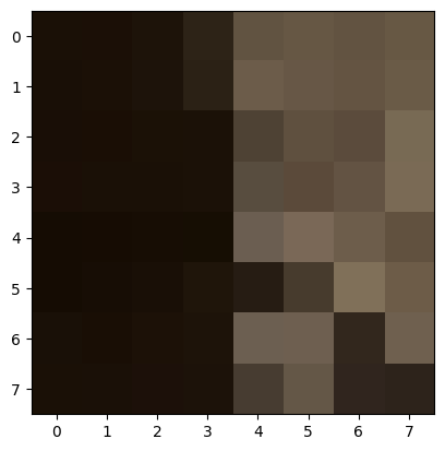
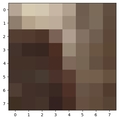
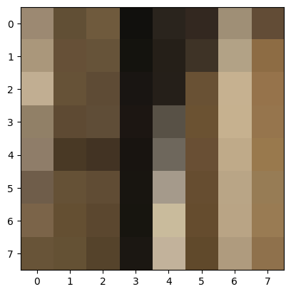
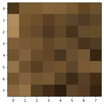
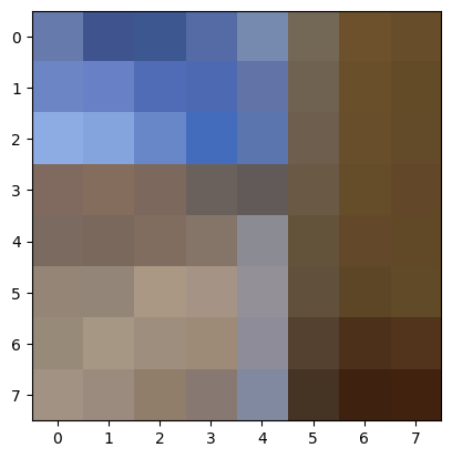
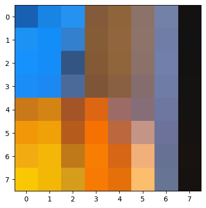
After obtaining 8x8 patches for all candidate points, I then match them with the 8x8 patches of candidate points on the other image using an SSD metric. For each candidate point p in the first image, I find the nearest neighbor and the second nearest neighbor. Two points are nearest neighbors if their 8x8 patches have the lowest SSD value out of all other pairings (with the first image’s point). The second nearest neighbor is calcualted in a very similar way (using the second lowest SSD value).
Once the first nearest and second nearest neighbors are calculated for point p, I then calculate the ratio 1-nn/2-nn. Here, 1-nn and 2-nn correspond to the SSD values between p and the nearest/second nearest neighbors, respectively. If this ratio turns out to be below some threshold (which I set to 0.3 by default), then I decide to keep point p and its nearest neighbor. The idea is that if the 1-nn is a better match than the 2-nn by a large enough difference, then we have a real match between point p and the 1-nn neighbor.
If the ratio does not meet the threshold, then we remove point p out of consideration.
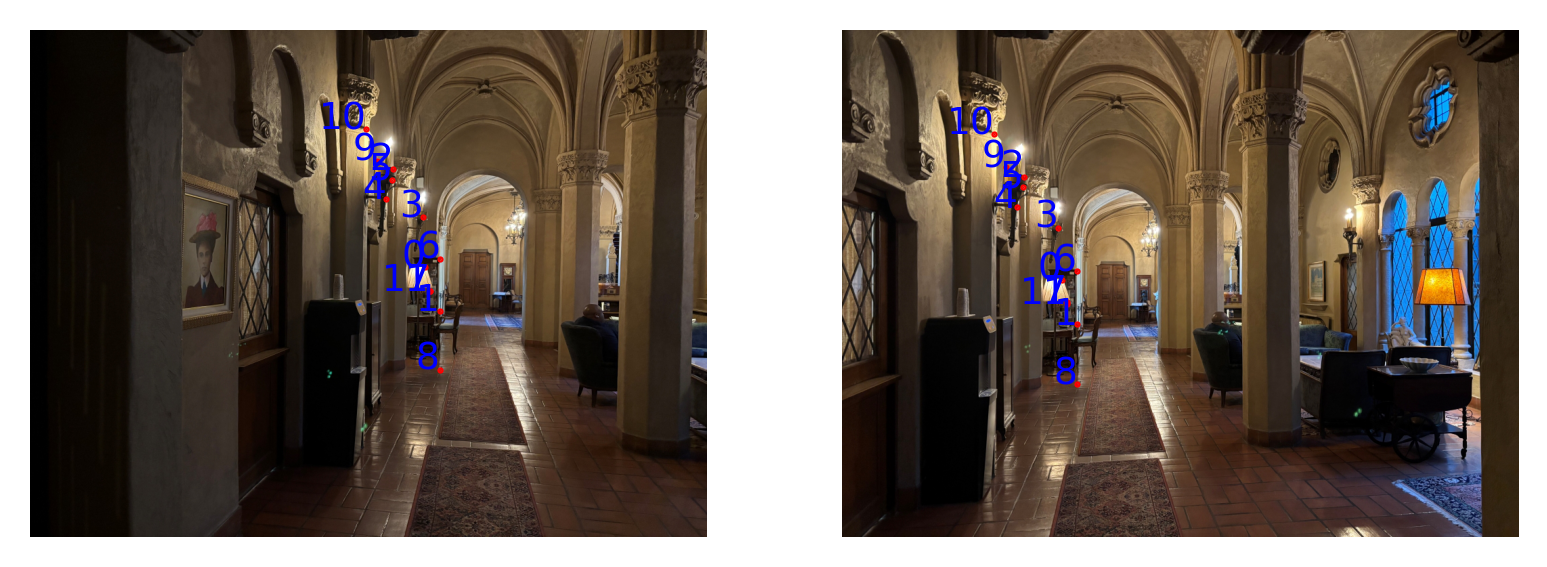
On top of feature matching, we also use RANSAC to further filter out points that don’t match well. The process is as follows:
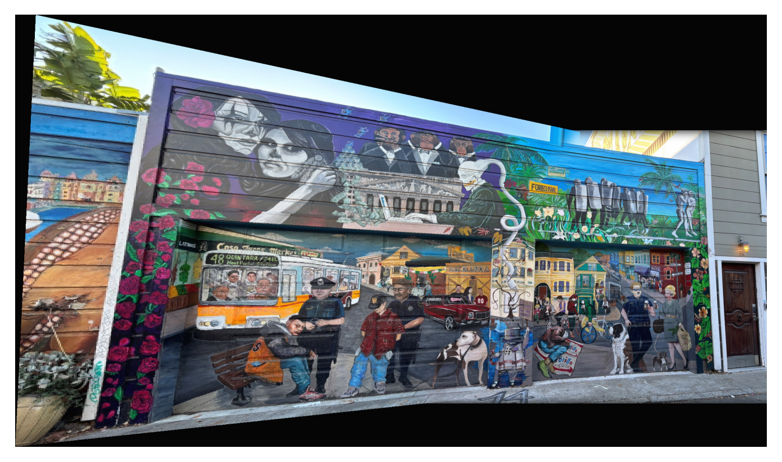
We use the largest set of inliers as our final correspondence points for computing a homography and warping images to build a mosaic.
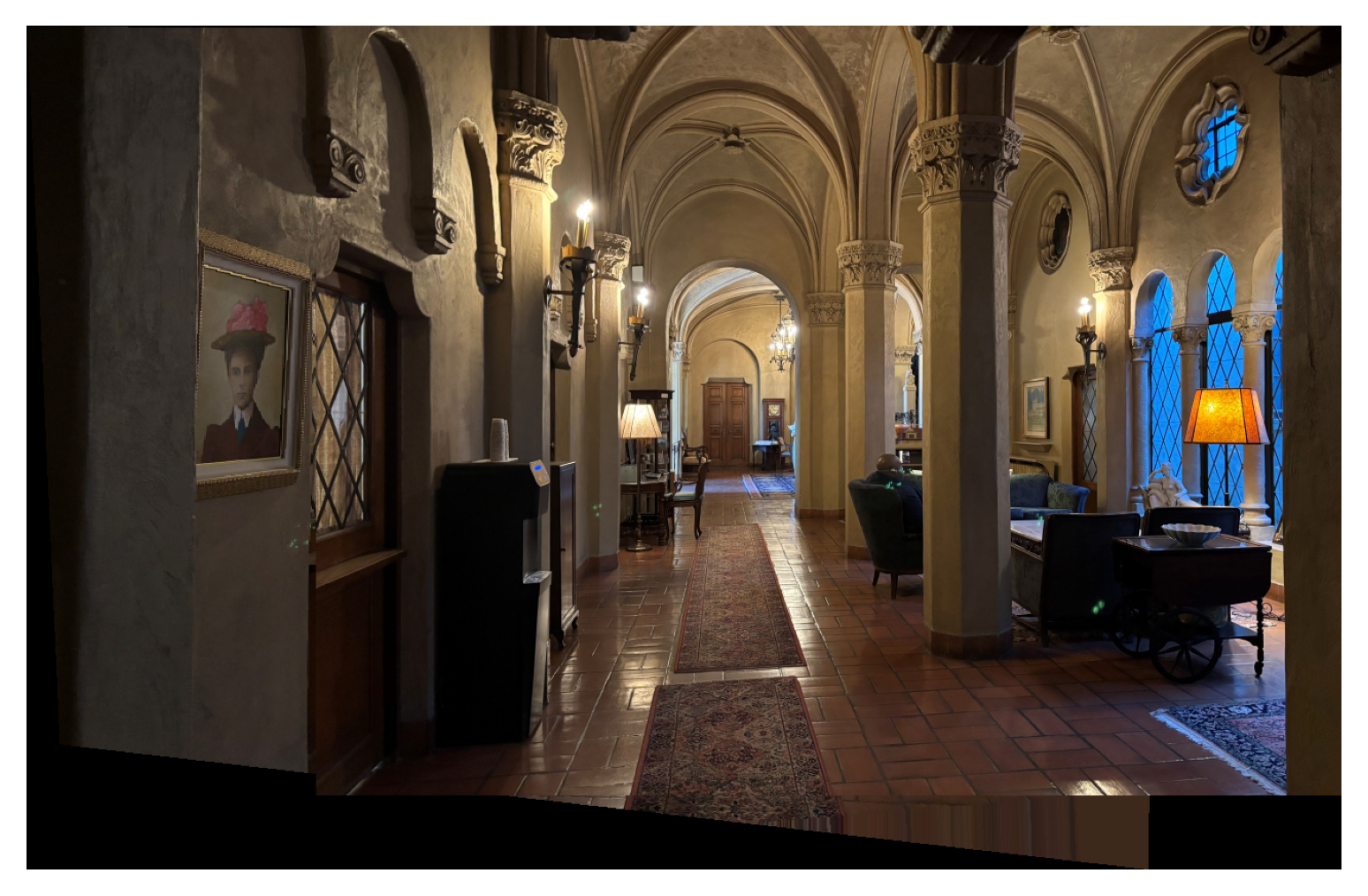
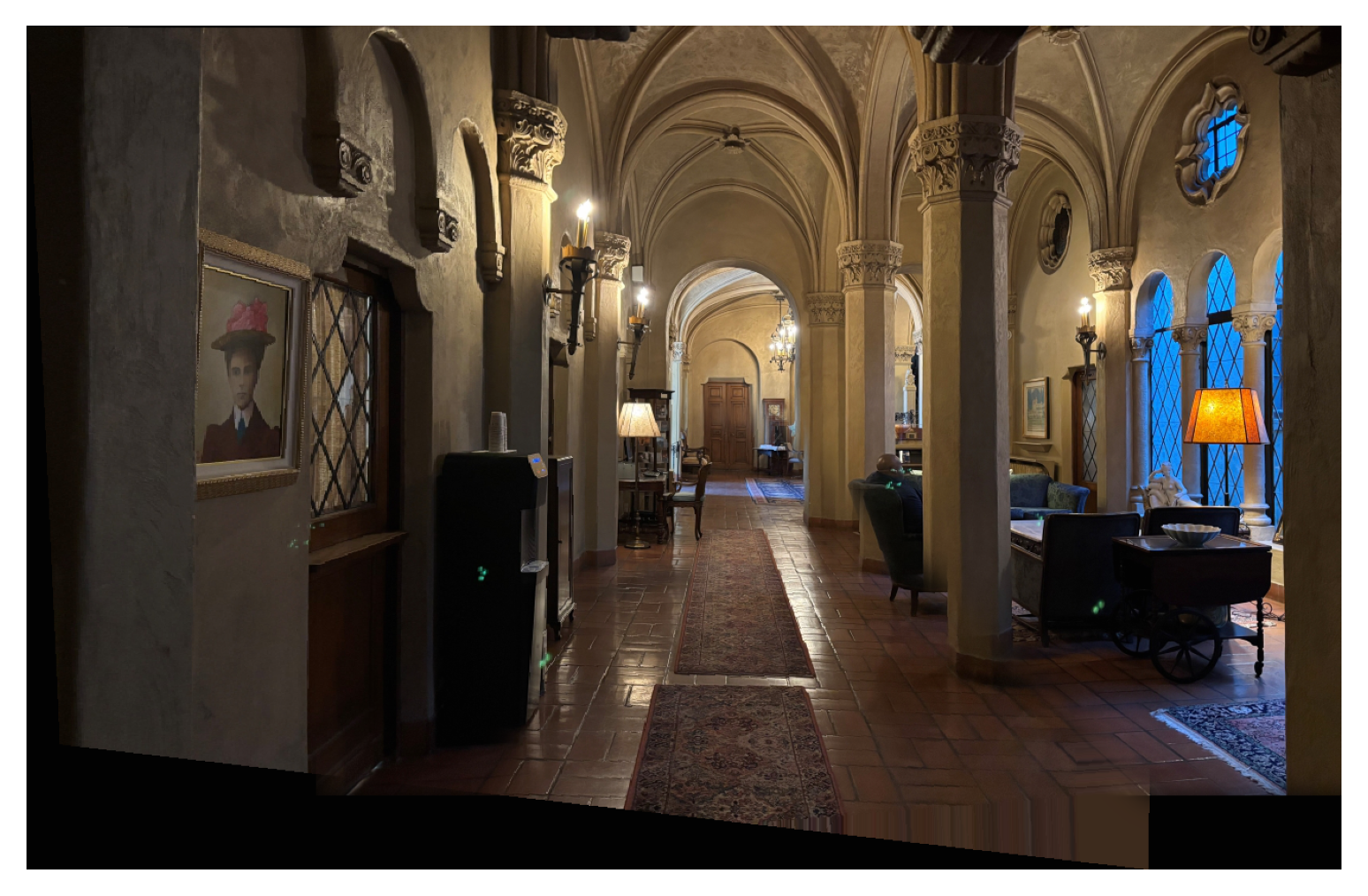
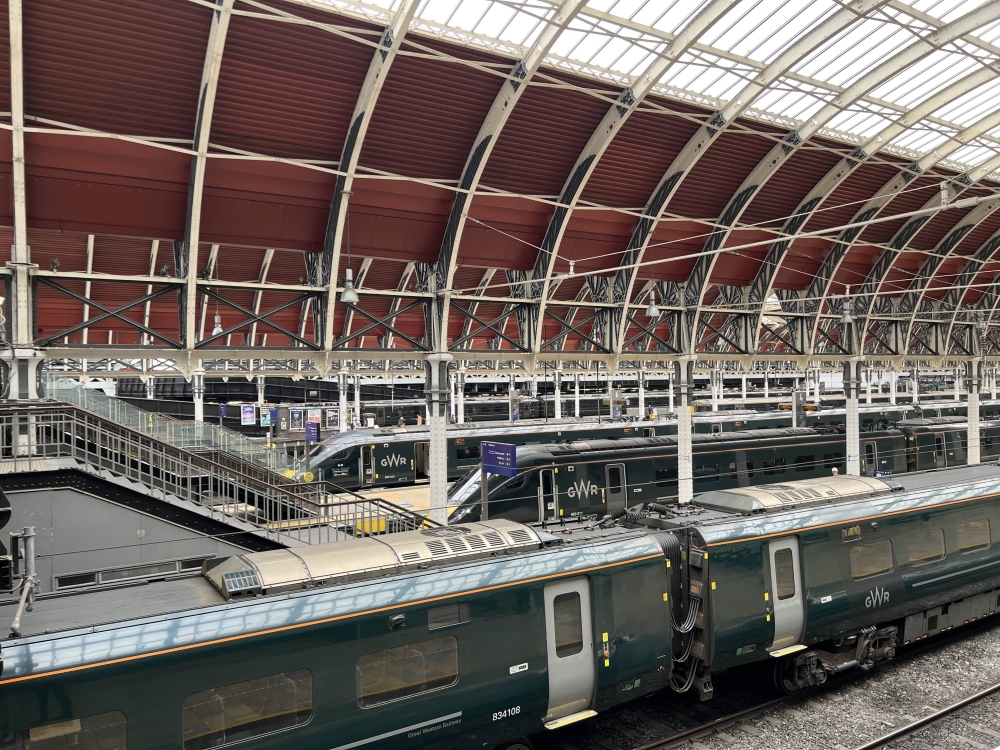
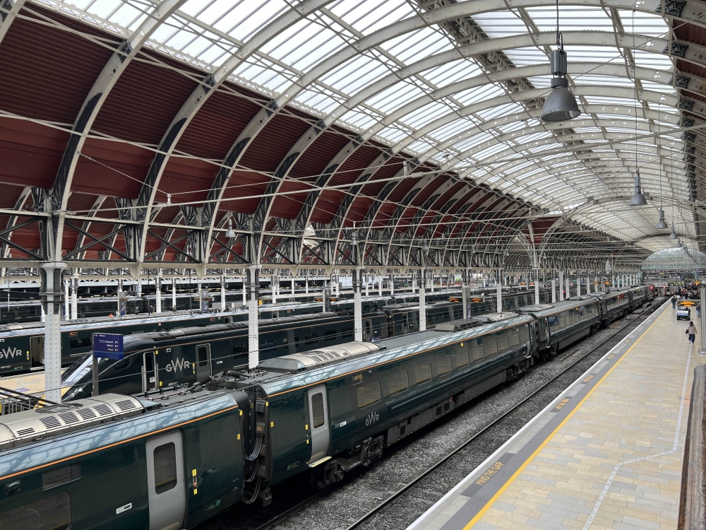
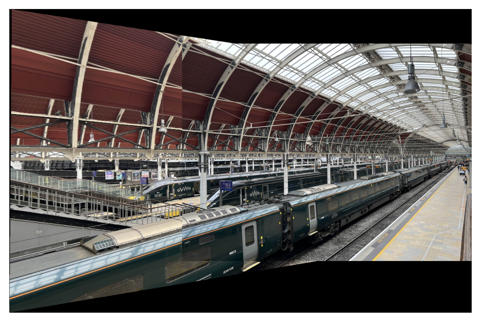
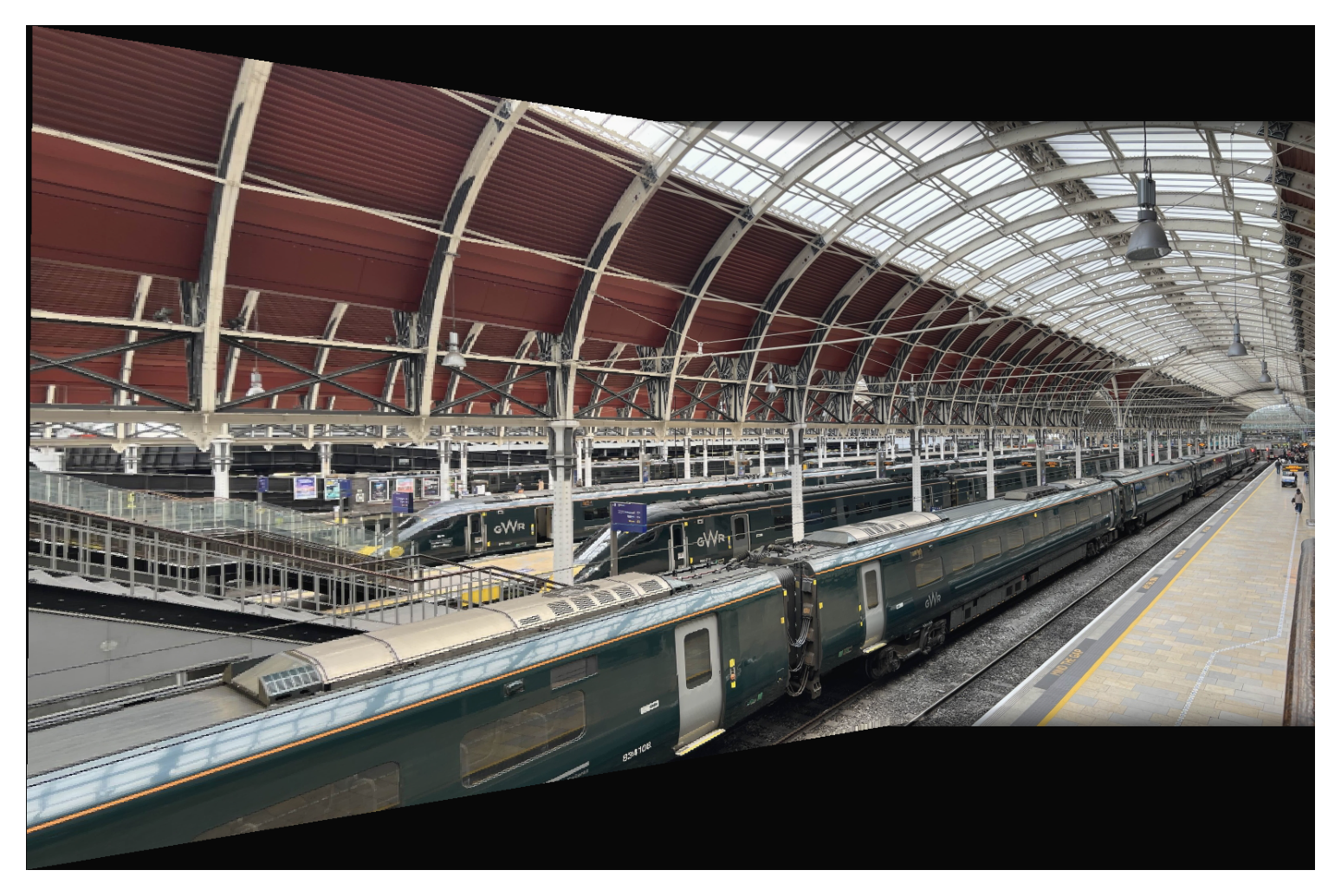
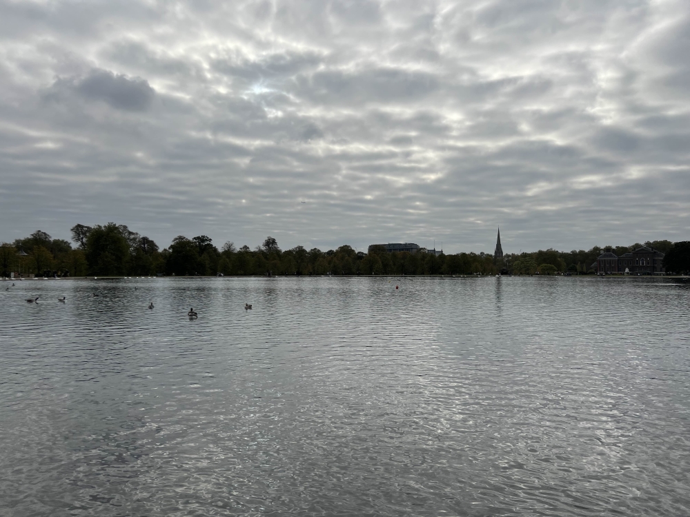
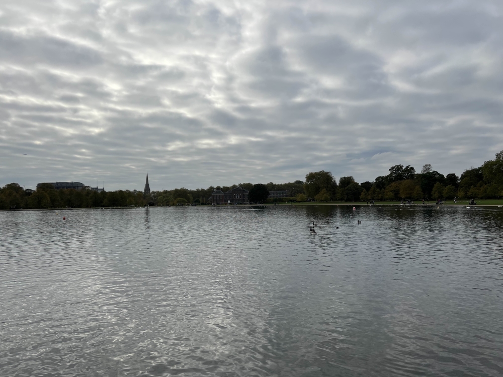
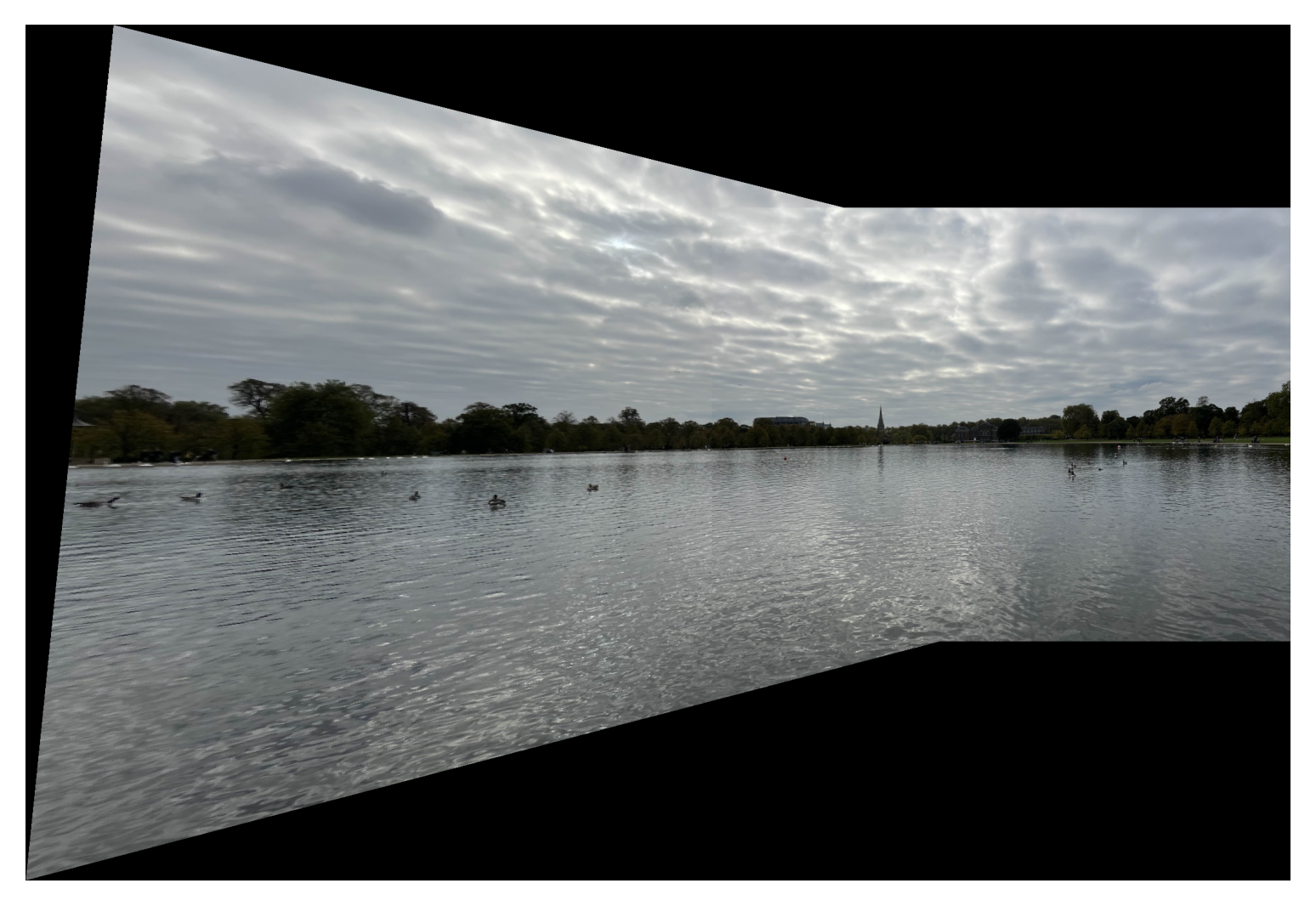
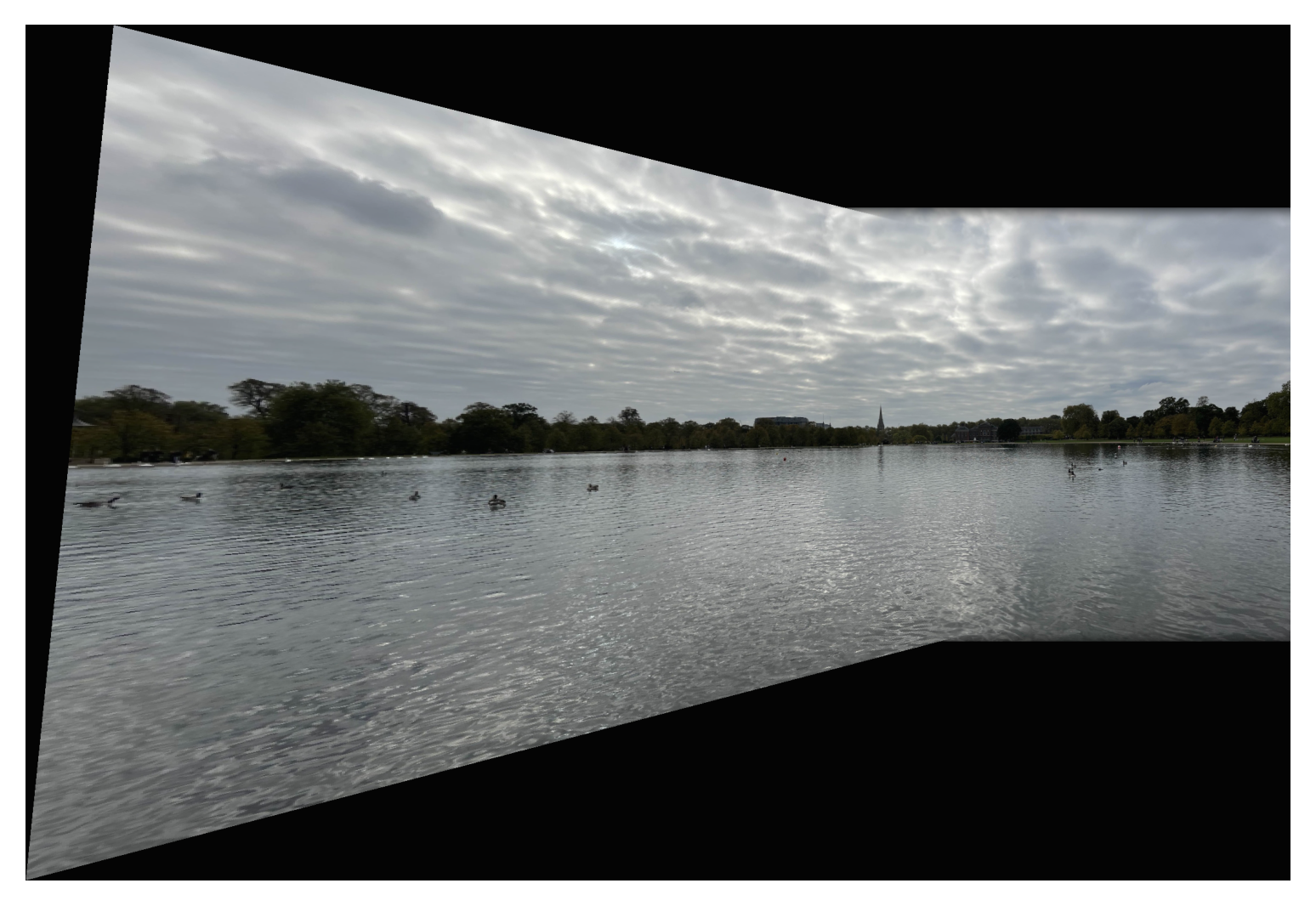
Even though autostitching and RANSAC was fun to implement, I think the coolest part of the project was image rectification. Image rectification took me the longest to implement, and when it finally succeeded, I was very happy. Getting image rectification down also made image mosaicing later on less complicated.