Final Project(s)

Fall 2024

1. Light Field Camera

In this part, I take data from a light field camera to simulate image focusing. I also simulate aperture adjustment to create different levels of depth of field.

To focus certain layers of an image and blur other parts, I take the average of a grid of images taken at slightly different angles/positions. To change the focus, I shift each image based on their relative position from the reference image in the center of the image grid. After calculating this shift, I multiplied by a constant c. Adjusting c adjusts our layer of focus on the image.

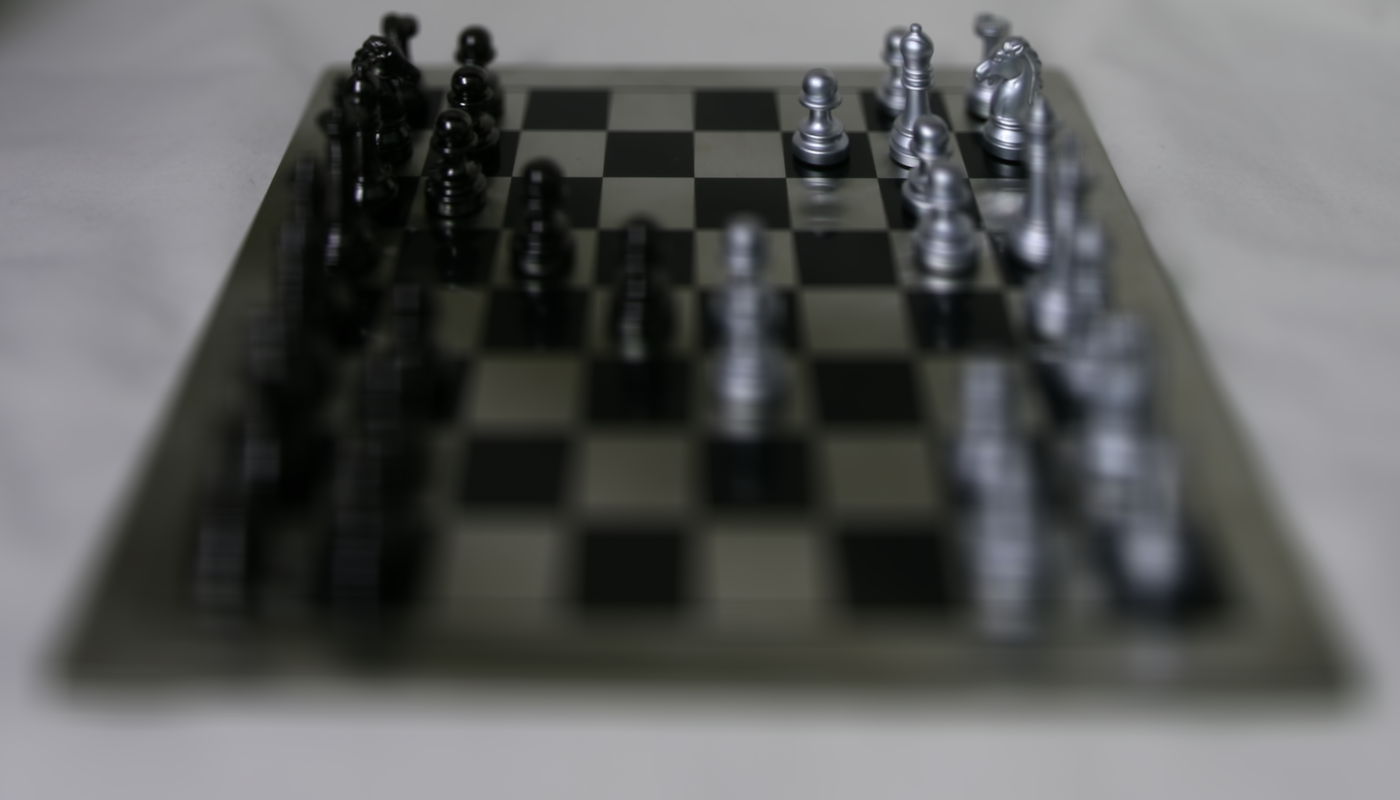
I implemented this on the chessboard image set. The set was a 17x17 image grid, where the image at [8,8] corresponded to our center image. After calculating the distance of each image from the center image, I multiplied each image by c. I found c values from [-0.2,0.7] to best capture the entire depth of the chessboard. Lower c values focused on the farther parts of the board, while higher c values focused on the closer features.

c = 0

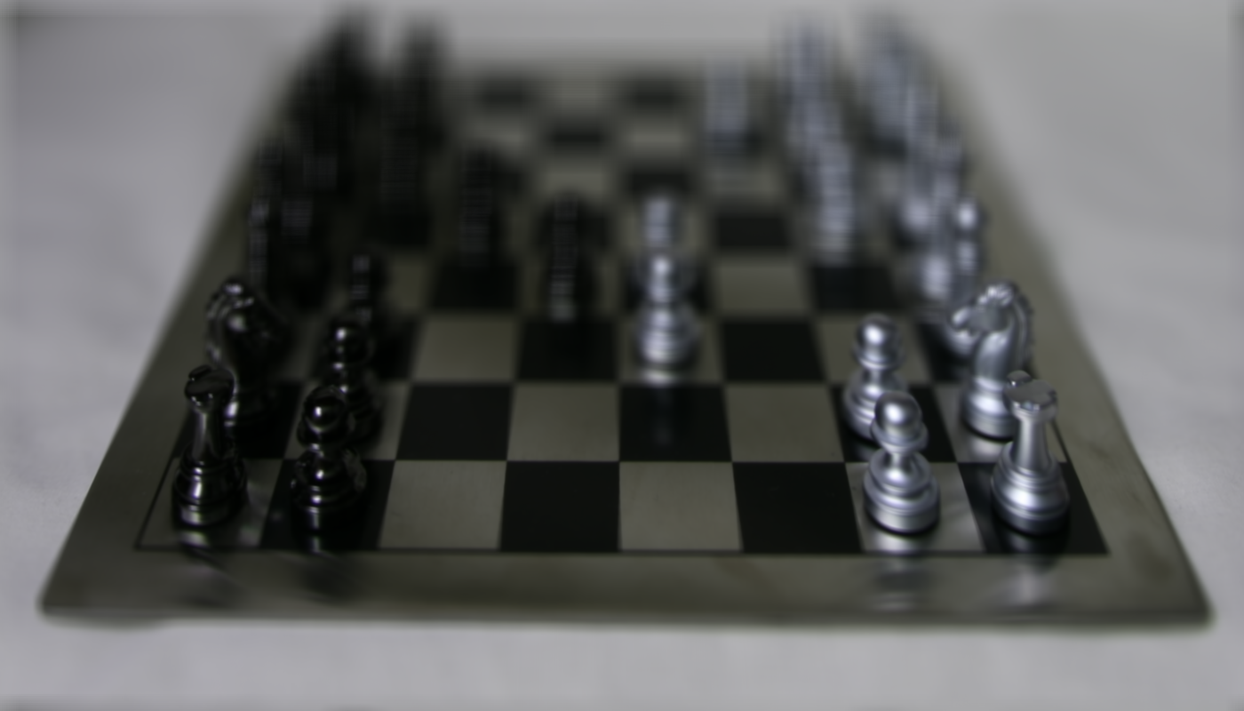
c = 0.5

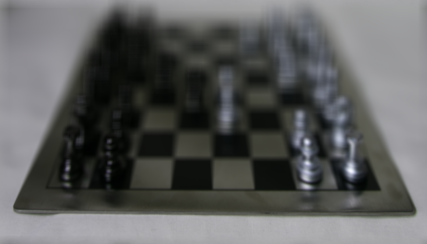
c = 0.7

Chessboard Image Refocusing GIF

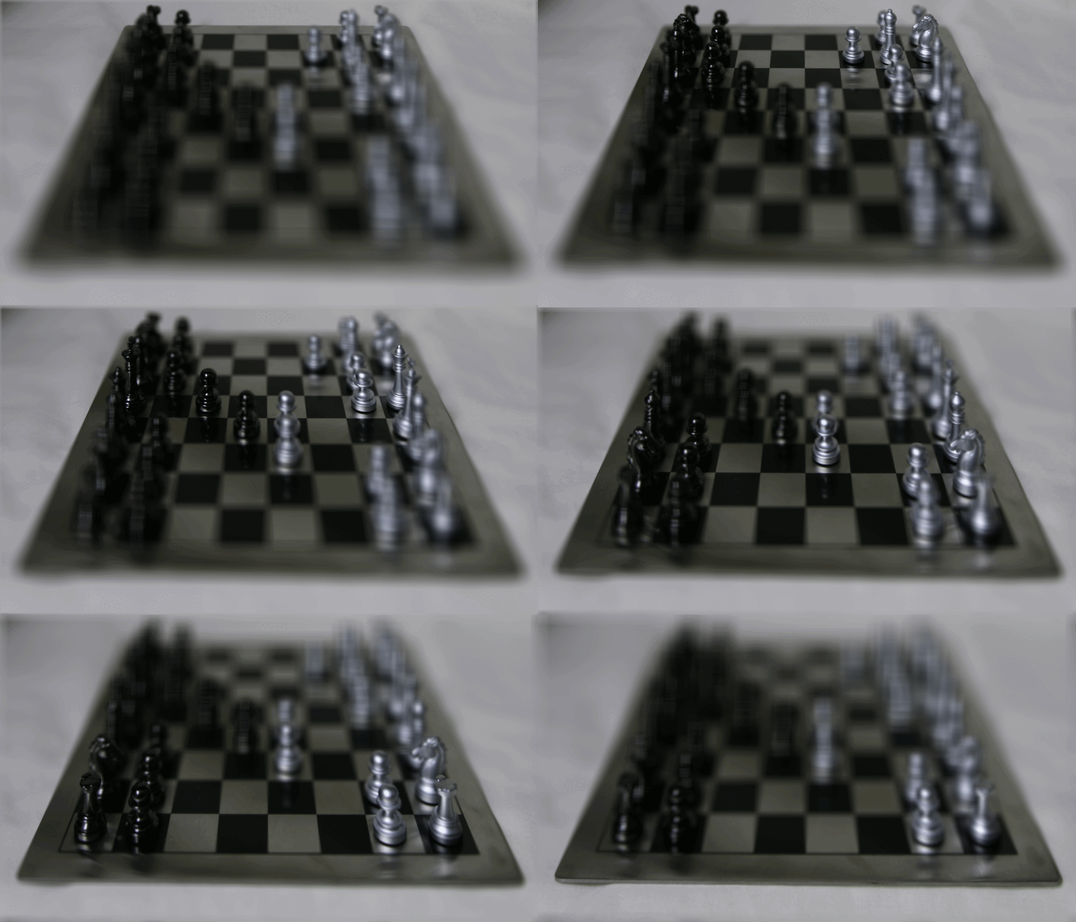
We can also simulate varying depths of field using light field data. While keeping c constant, we can adjust the number of images to average. For instance, a window size of [-2,2] would include the images within 2 units to the left and right of the center image.

A smaller window corresponded with a smaller aperture and deeper DoF, while a larger window corresponded with a larger aperture and shallower DoF.

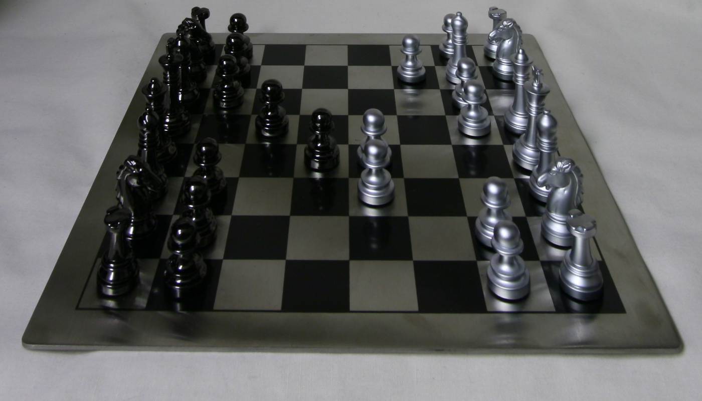
window = 0

window = [-4,4]

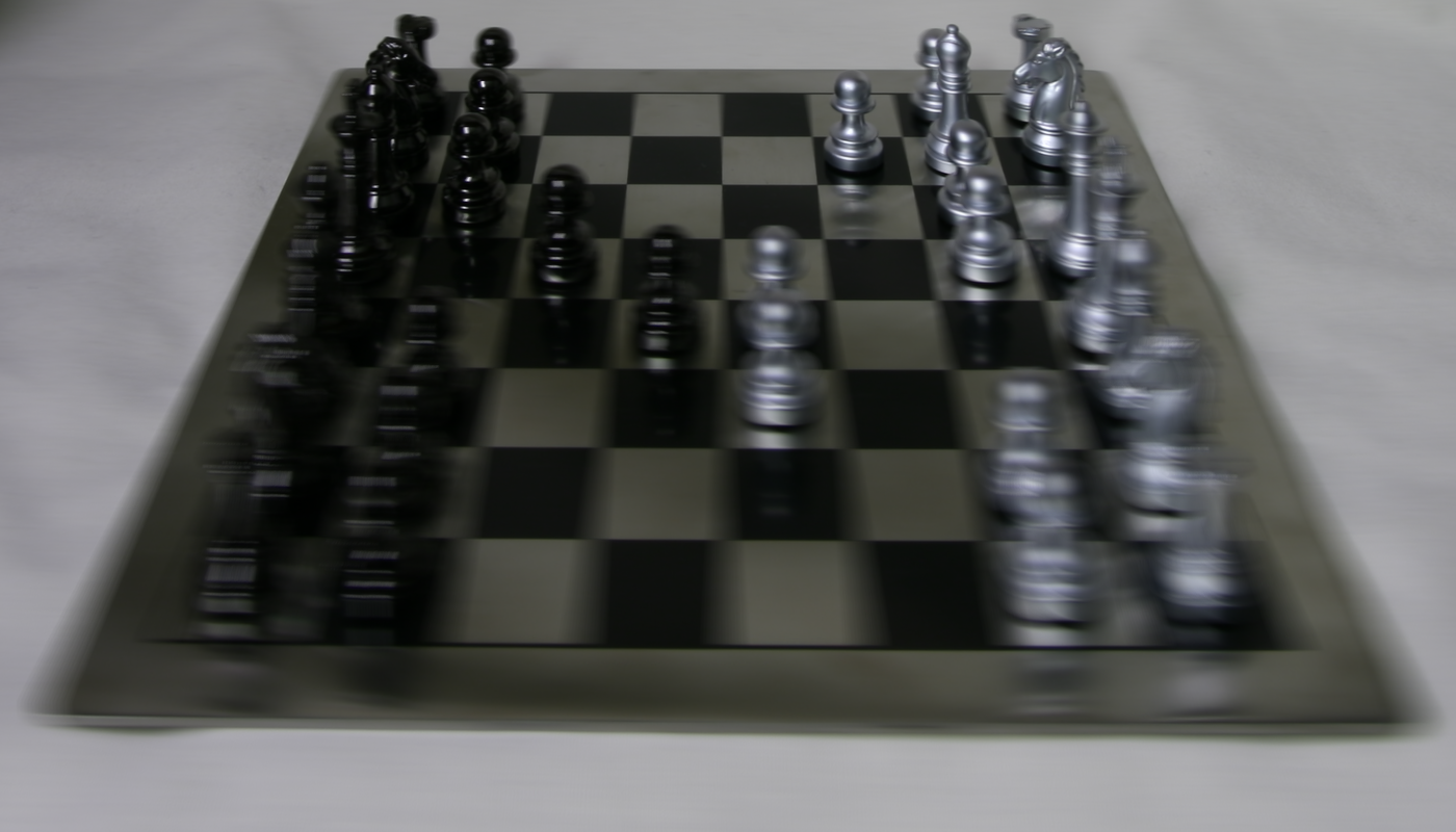
window = [-8,8]

Aperture Adjustment GIF, c=0

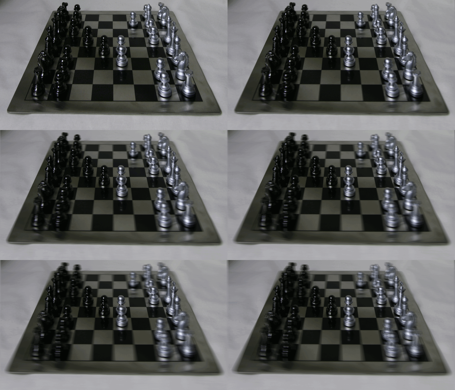
c=0.2

2. High Dynamic Range Imaging

For this part, I implement high dynamic range (HDR) to adjust images for differences in image exposure levels. If we take a picture at multiple exposure levels and apply HDR, we can create a higher quality photo that can show details in both light and dark areas.

To create the radiance map of a set of images at different exposure levels, we need to apply the following equation to each pixel i:

Z_ij = observed pixel value at position i for the jth exposure image

ln(delta t_j) = log shutter speed for the jth exposure image

w[Z_ij] weighs each exposure image’s contribution to the final pixel value, allowing for higher estimation accuracy. Each pixel value is weighed differently, hence the index value Z_ij.

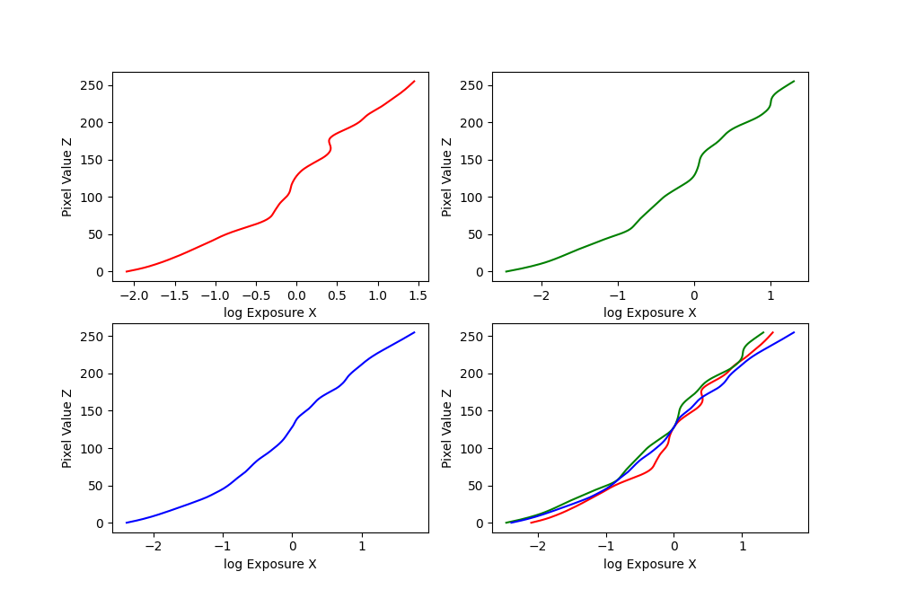
Our unknown variables are the response curve function g and the scene radiance Ei. g is defined as below:

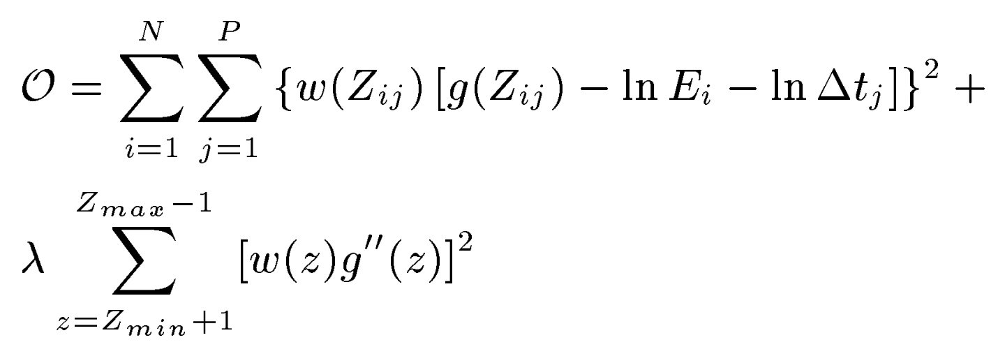
Fortunately, we can solve for g using the algorithm as described in the Debevec and Malik paper. Broadly speaking, we can construct a system of equations and use least squares to minimize the following loss equation (lambda represents a regularization smoothing term):

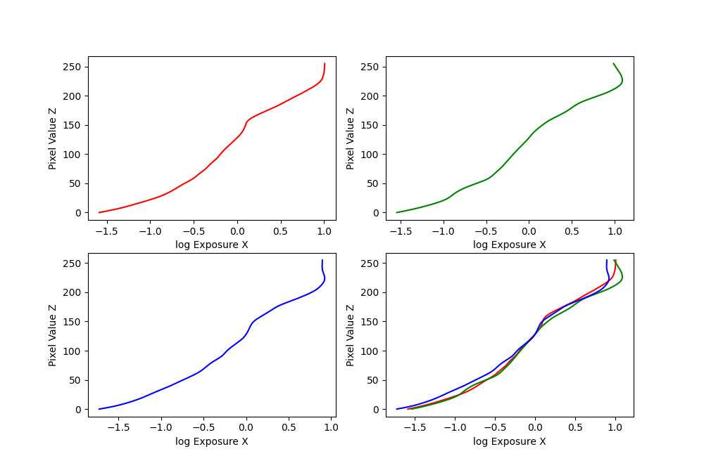
Resovered response curves for arch photo:

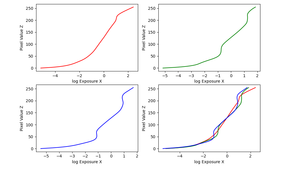
After recovering the g function for each color channel, we can use this to estimate radiance at each pixel, using the first equation shown above for ln(Ei).

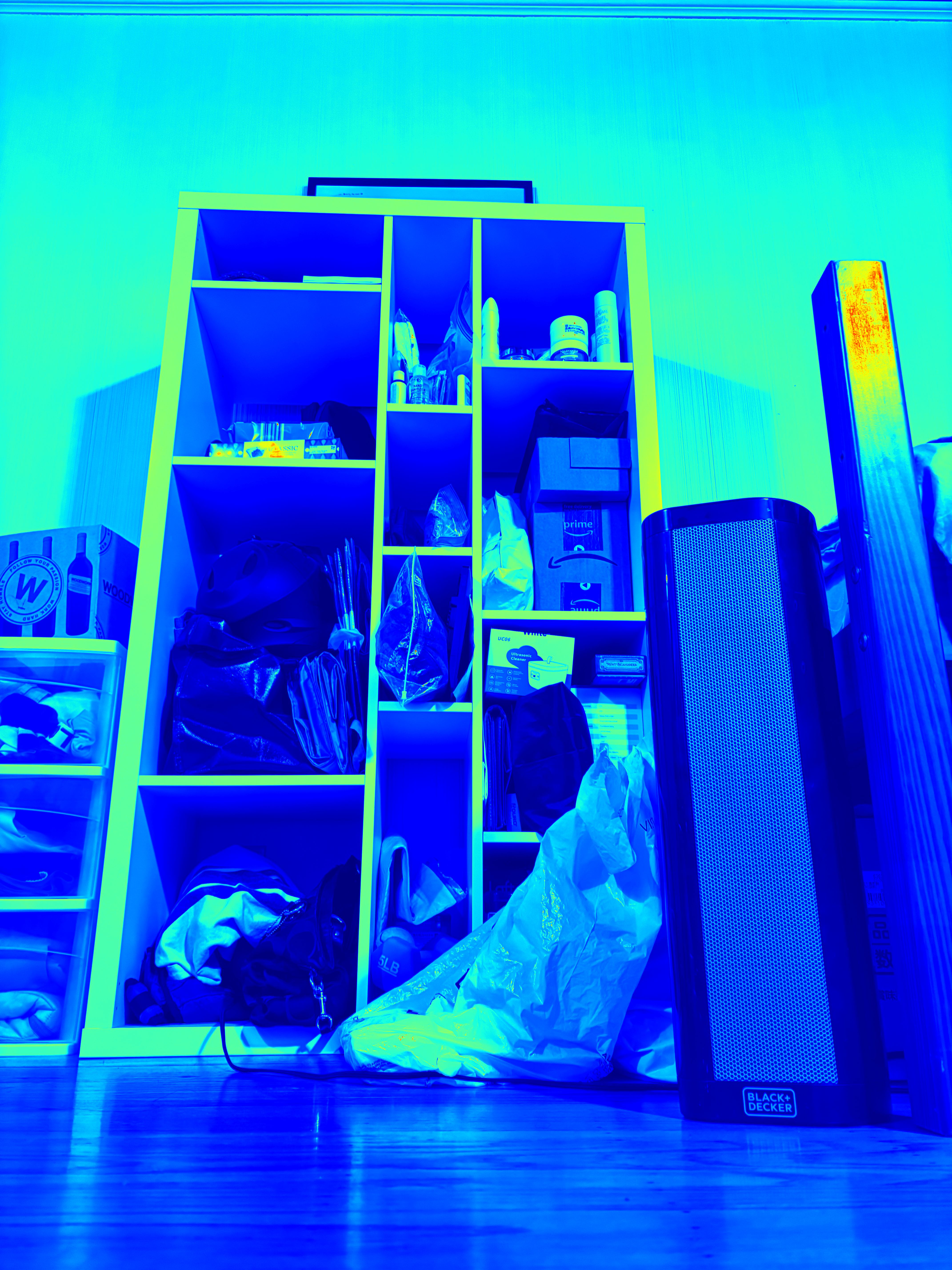
Calculating the log radiance and exponentiating the result for each pixel gives us the resulting radiance map:

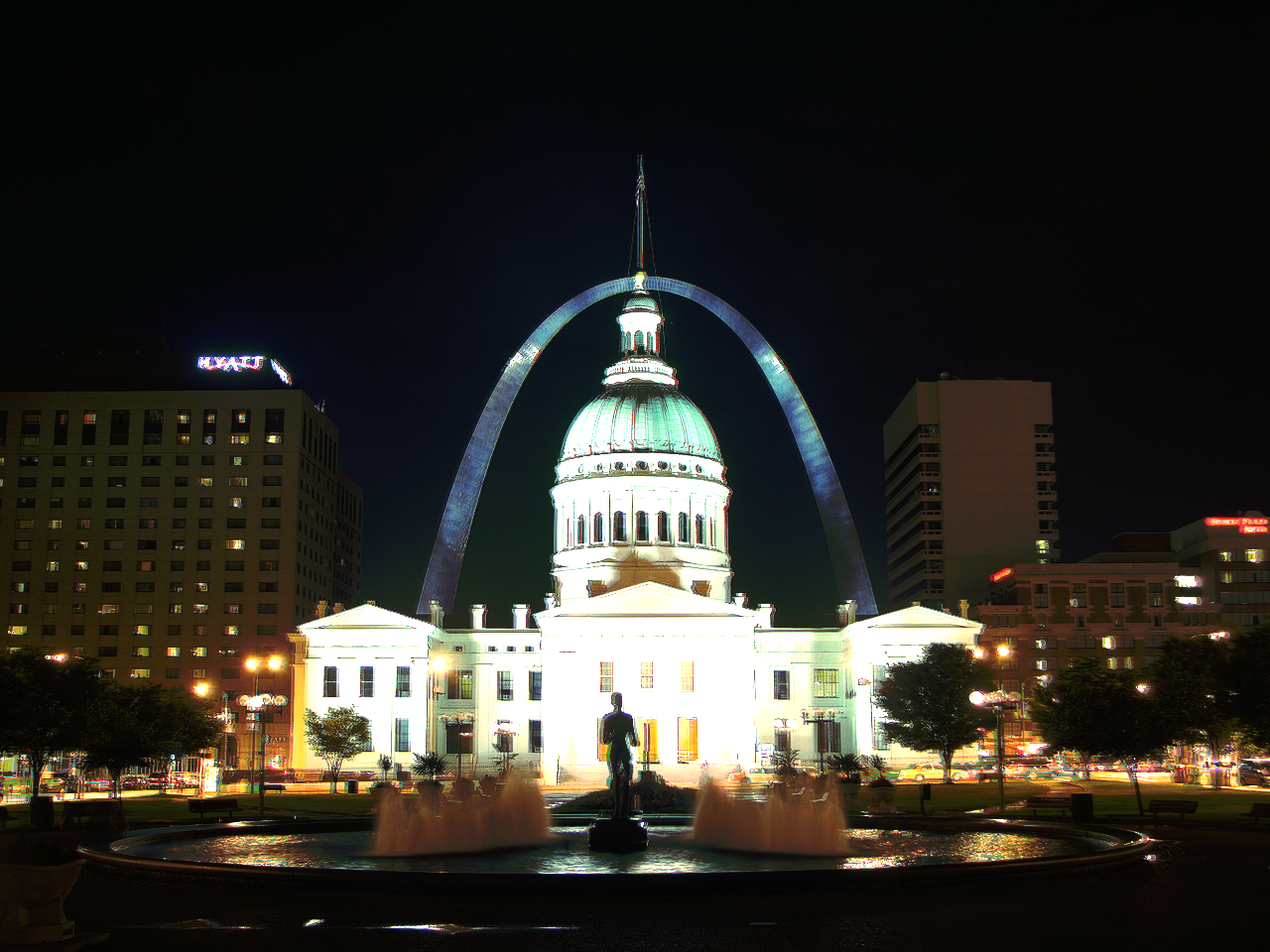
Radiance map

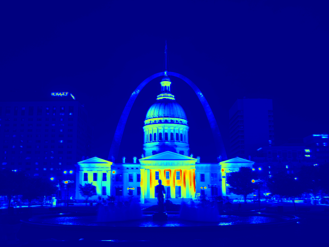
Averaged across all channels

By applying tone mapping, we can compress the dynamic range of the image to improve the details. There are three particular methods used here: global scale, global simple, and Durand.

The global scale method uses the min and max of the exposures to linearly scales the exposure values within the range of 0 and 1. When applied on the radiance maps, the resulting image usually turns out to be too dark.

The global simple method is a more improved tone mapping function, where for each pixel on the radiance map E_world, I calculate E_world / (1 + E_world). This often yields significantly better results than the global scale function.

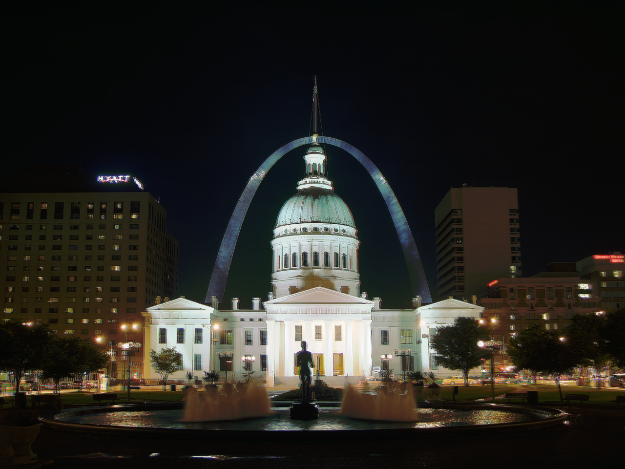
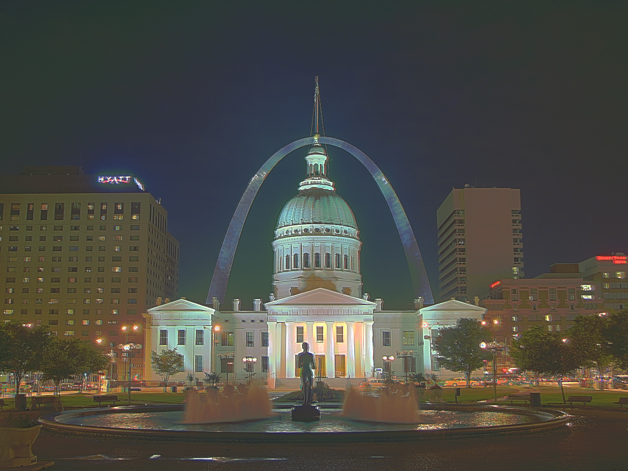
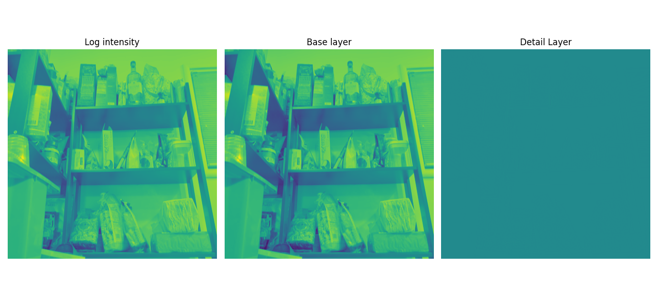
Additionally, I used Durand and Dorsey’s local tone mapping method. The Durand method results in an even more evenly lit image, often with the details accentuated. Without going into too much detail, this method generates a number of layers and recombines them a certain way to reconstruct the image.

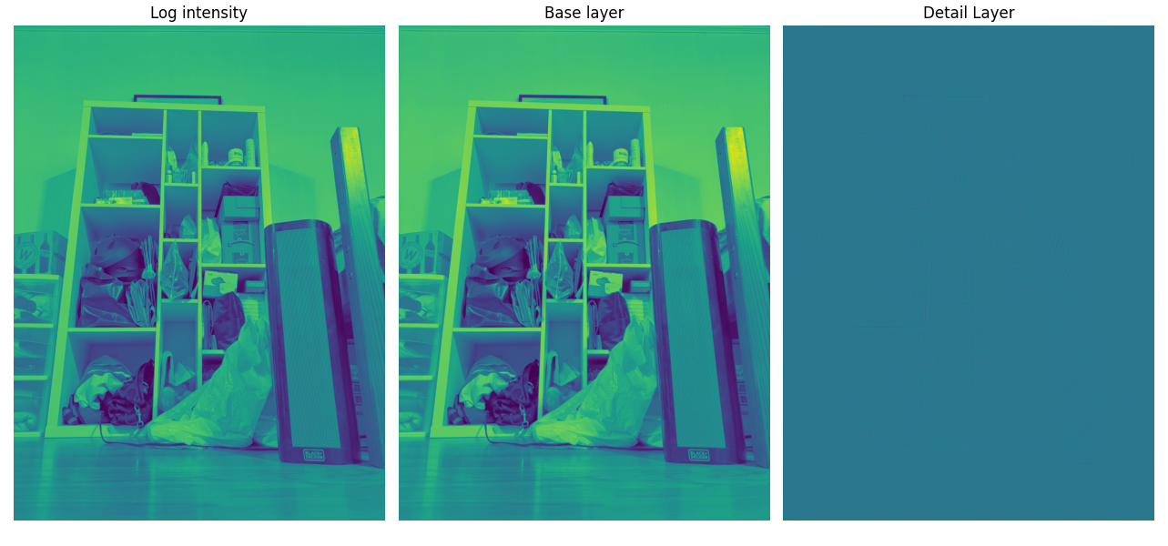
1. Average the radiance color channels to compute the intensity I, as well as the chrominance channels (R/I, G/I, and B/I).
2. Take log(I) and apply a bilateral filter to obtain the base layer.
3. Subtract the base layer from the log intensity layer to obtain the detail layer.
4. Scale and offset the base layer, then combine with the detail layer and chrominance channels to finally reconstruct the image.

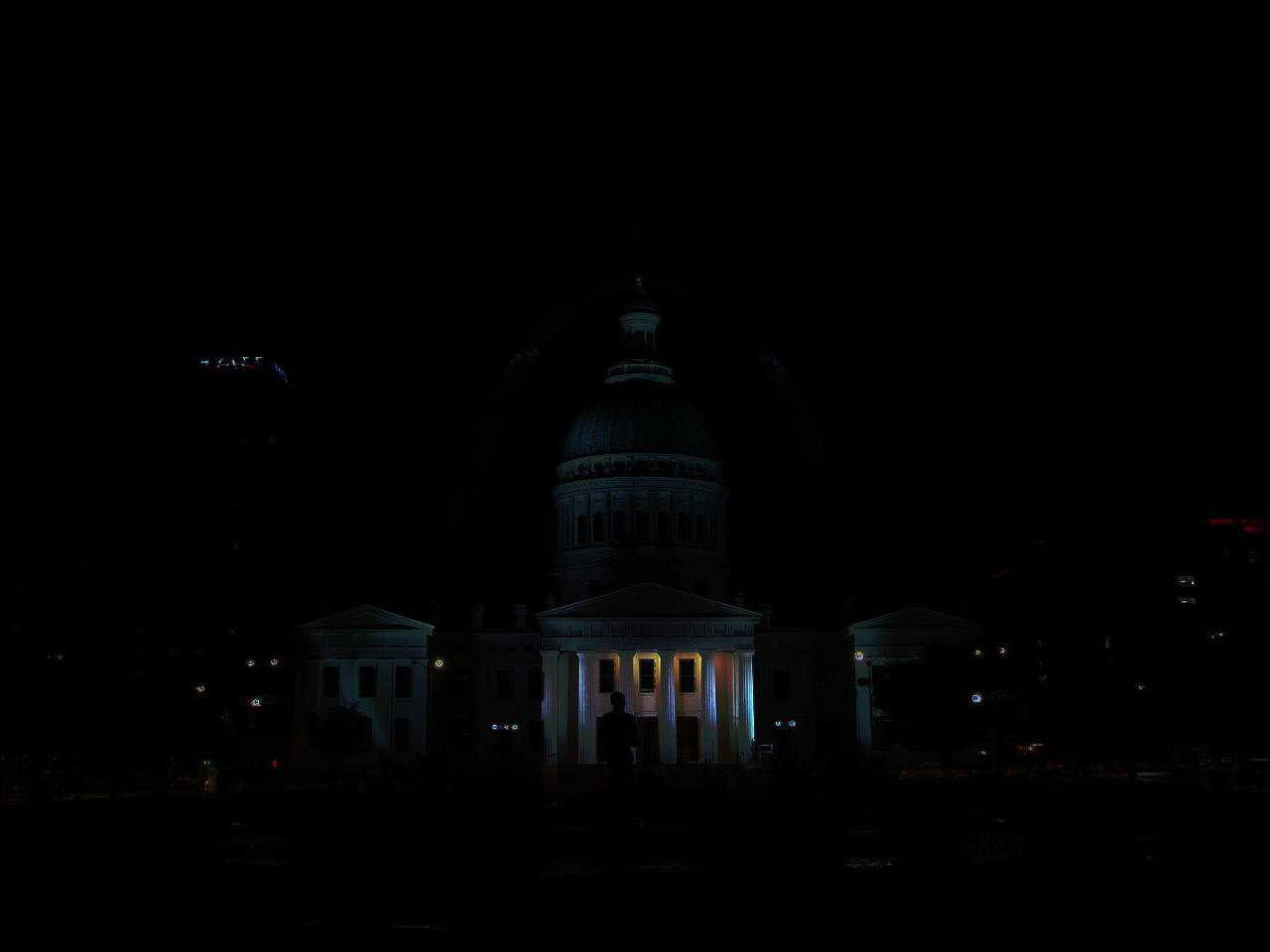
Log intensity, base, and detail layers for arch image:

Final result:

Chapel

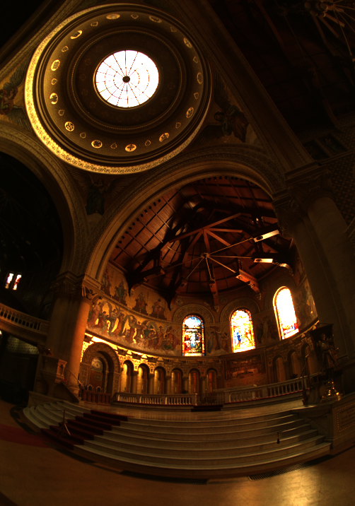
Radiance map

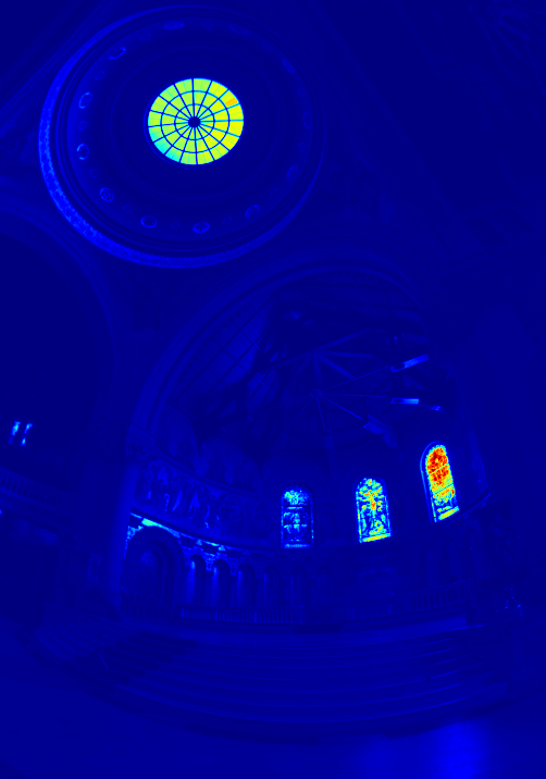
Averaged across all channels

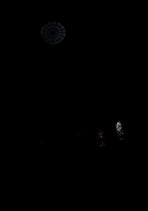
Global scale

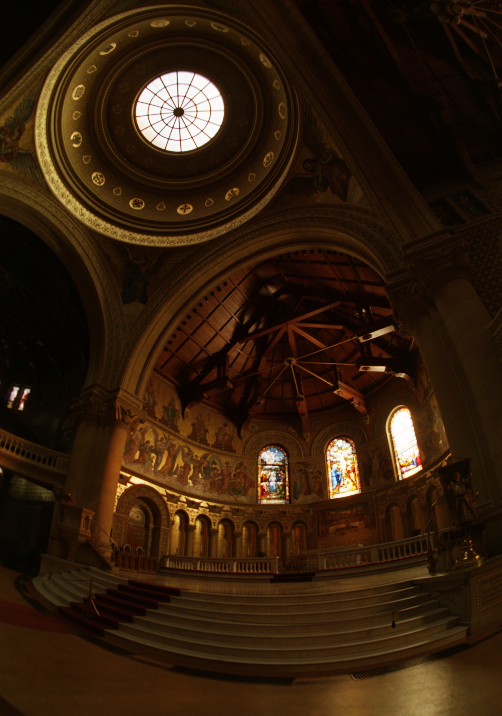
Global simple

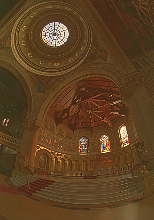
Durand

Bonsai

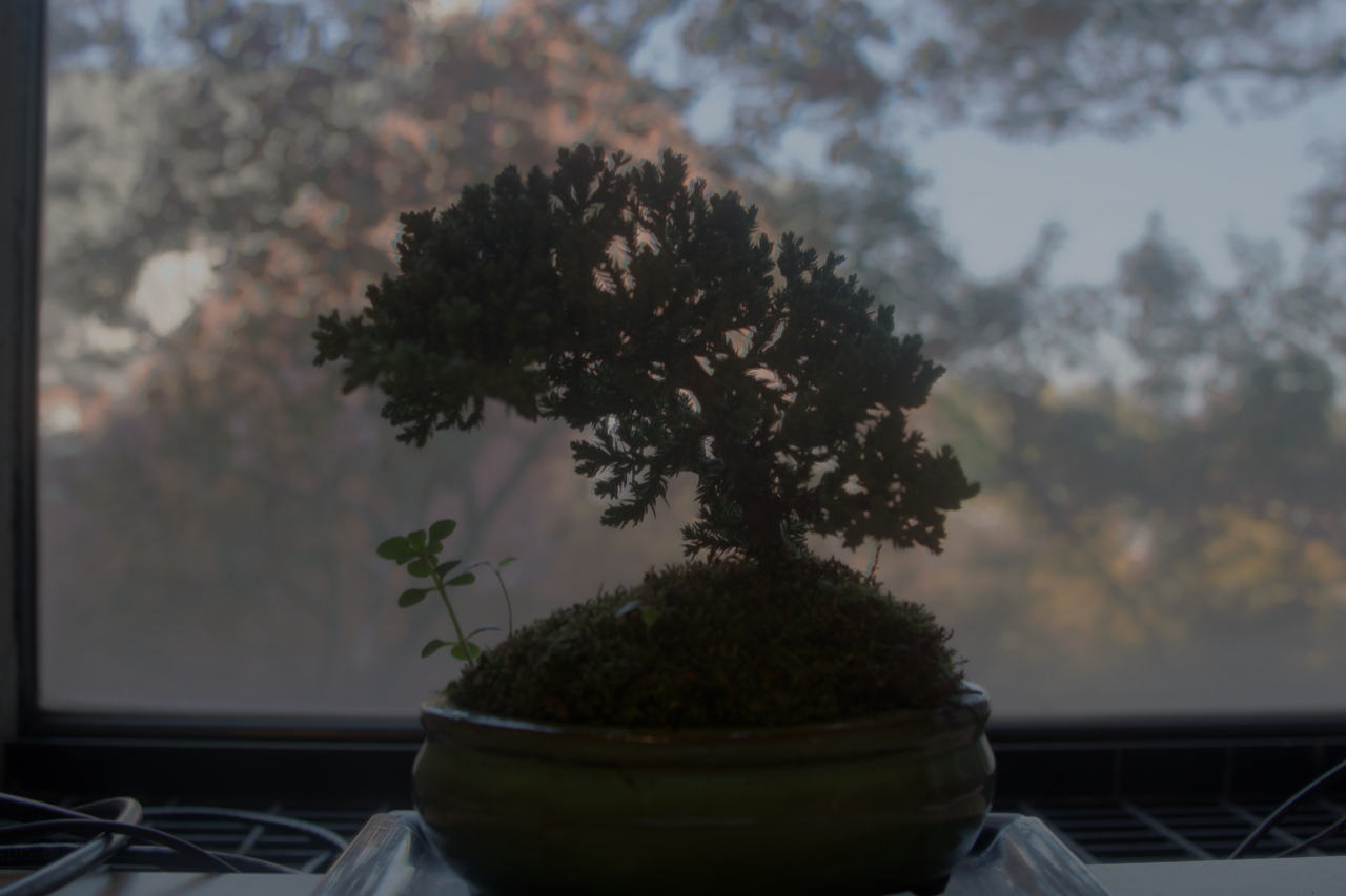
Radiance map

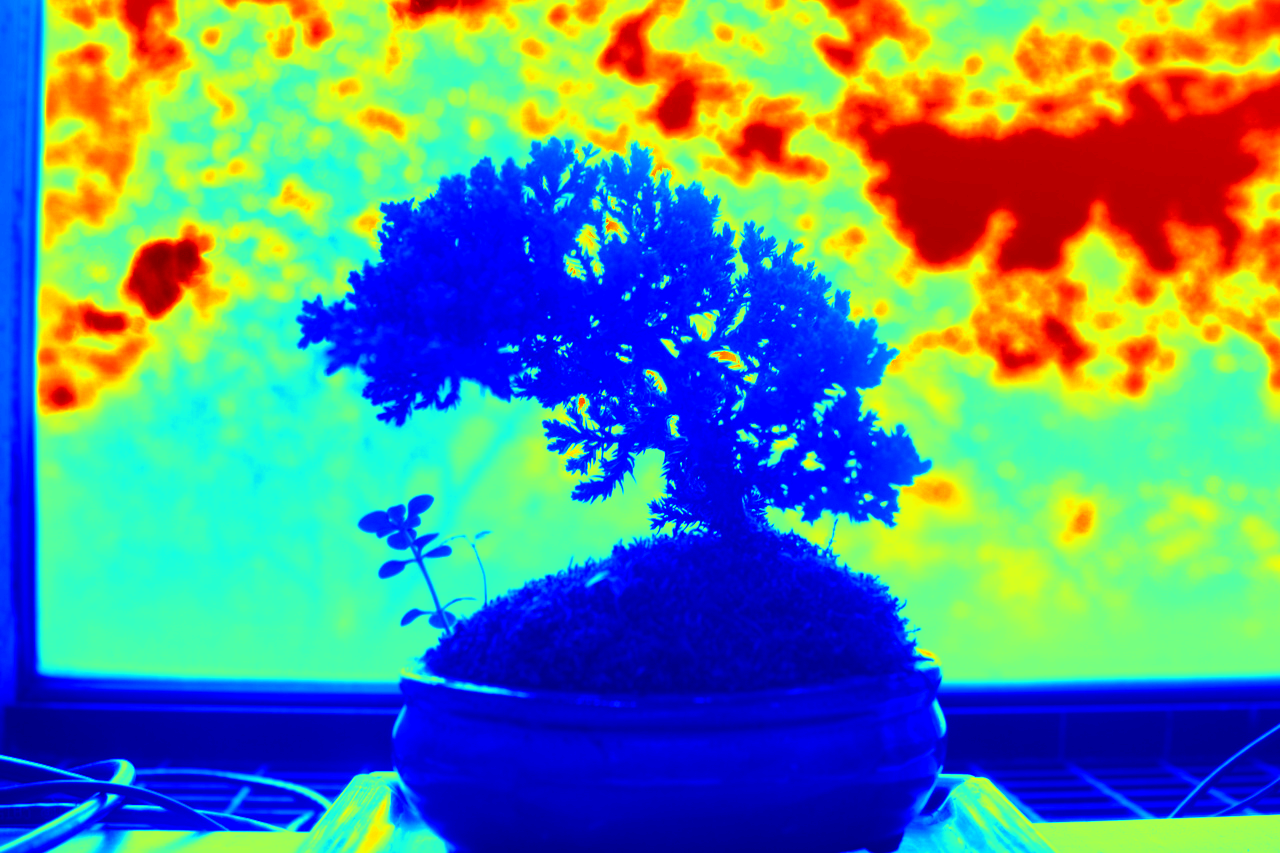
Averaged across all channels

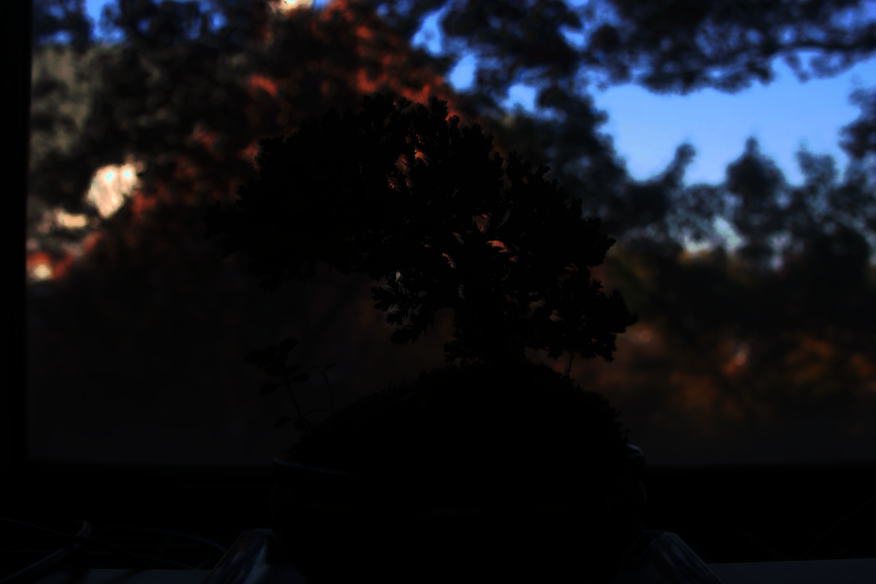
Global scale

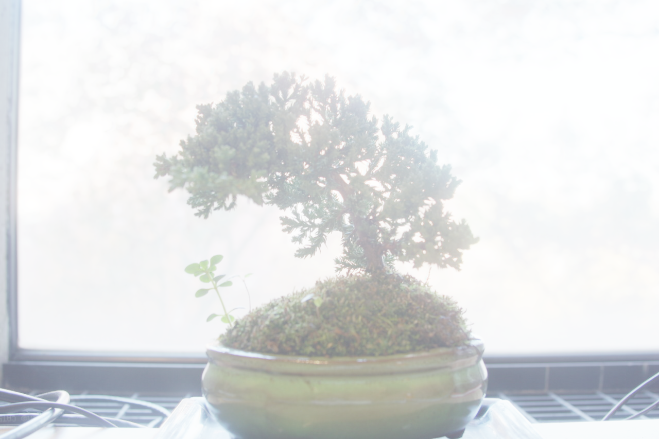
Global simple

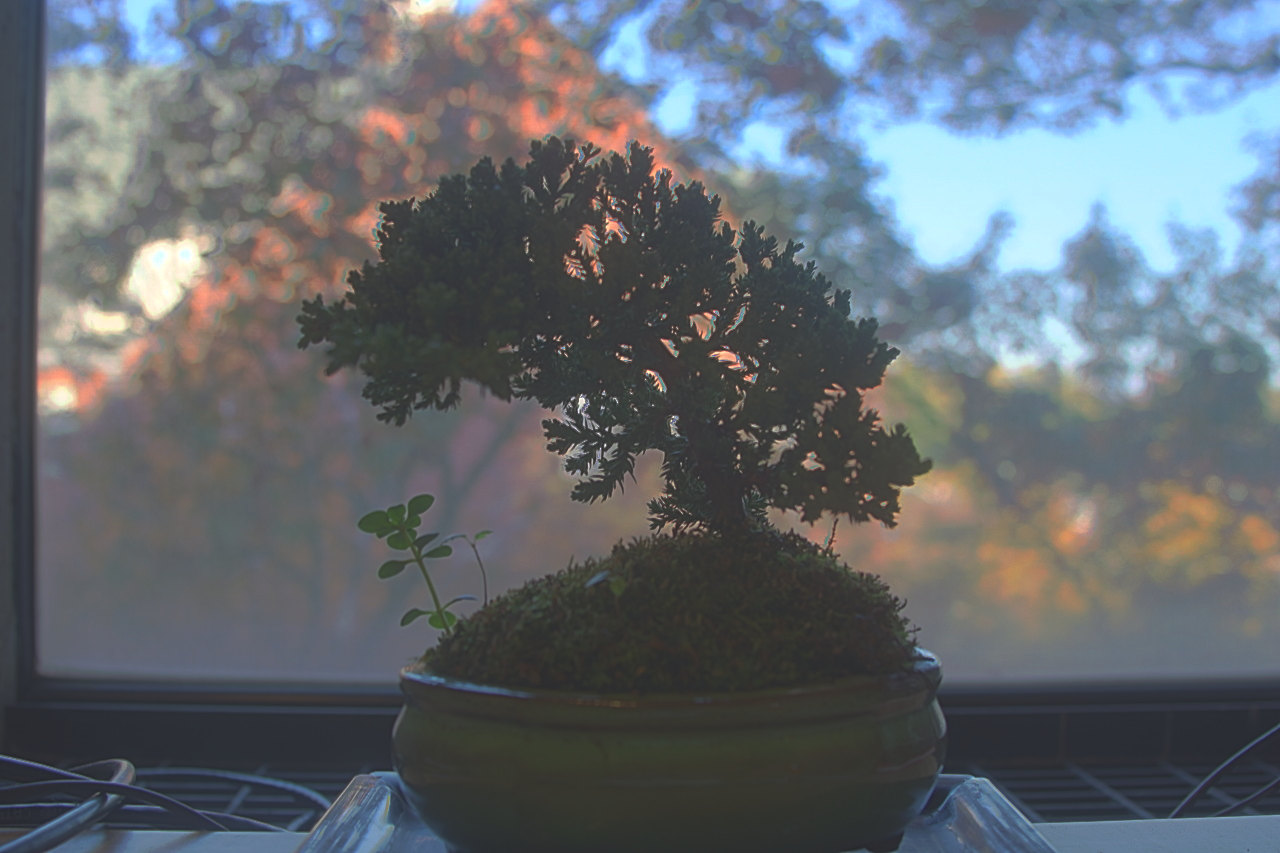
Durand

Window

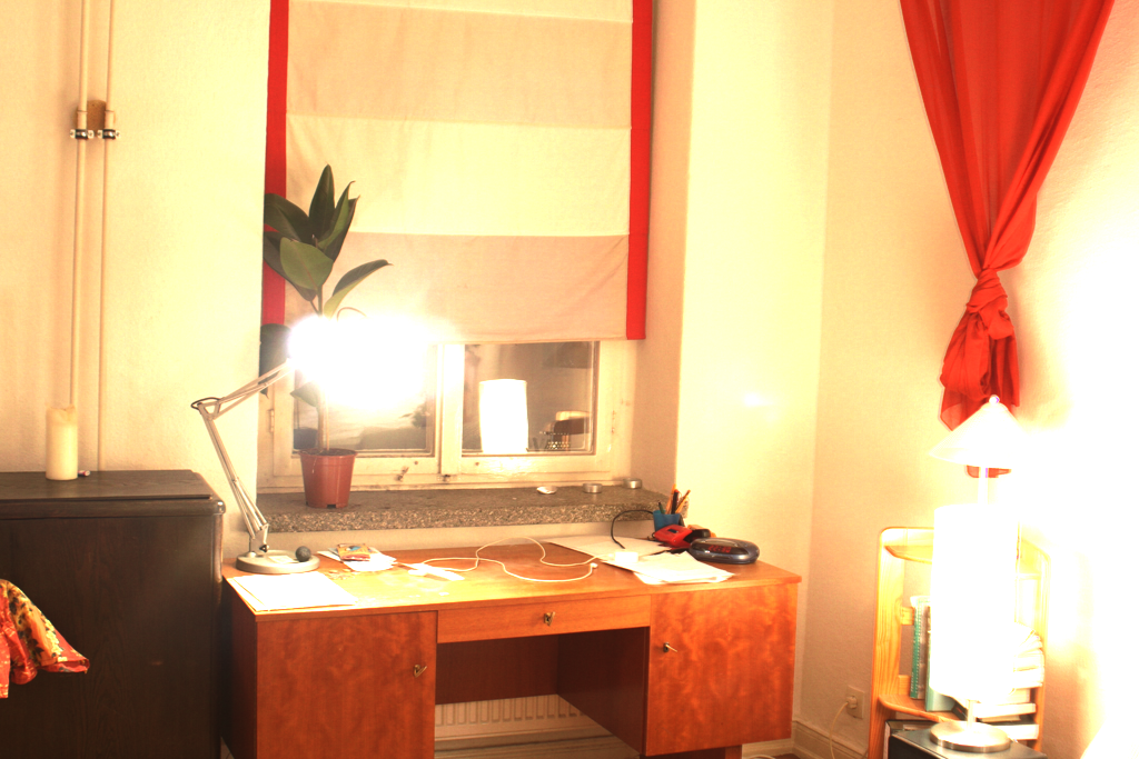
Radiance map

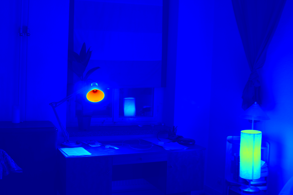
Averaged across all channels

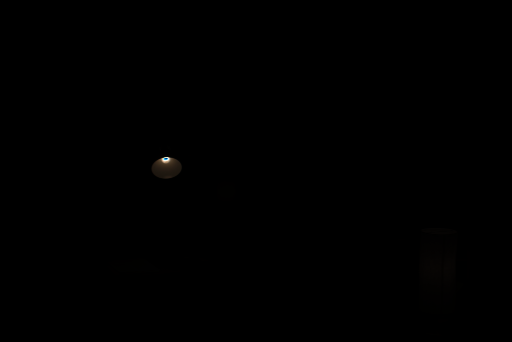
Global scale

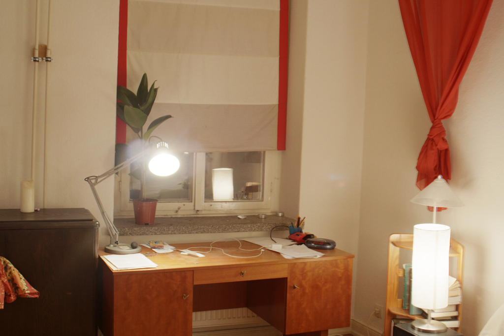
Global simple

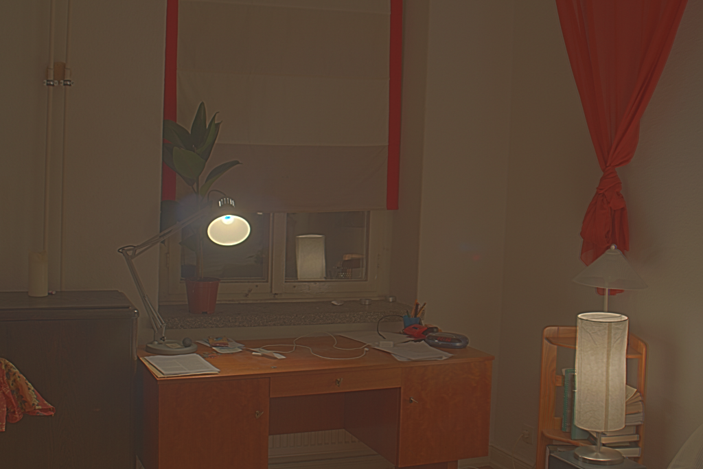
Durand

Mug

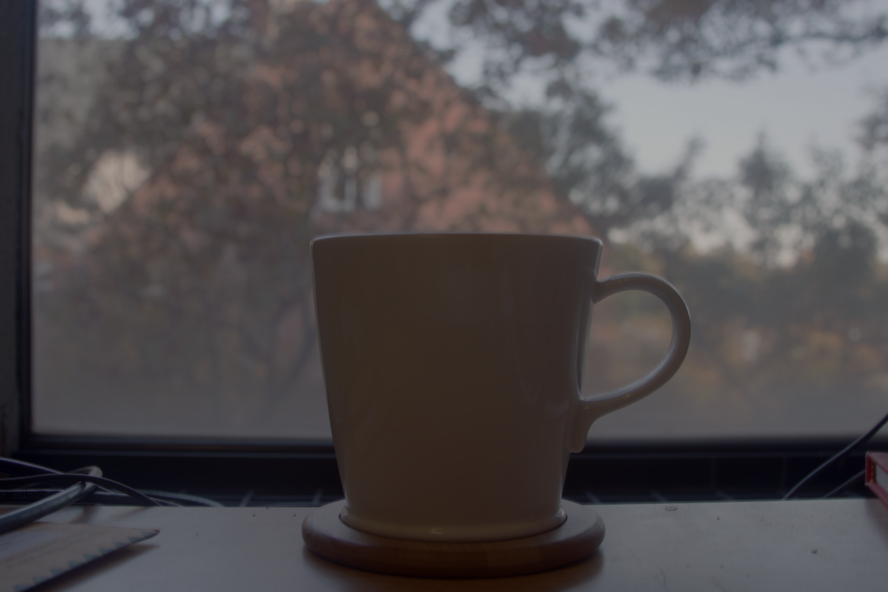
Radiance map

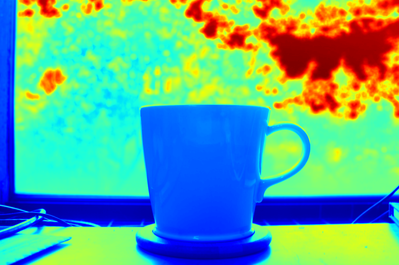
Averaged across all channels

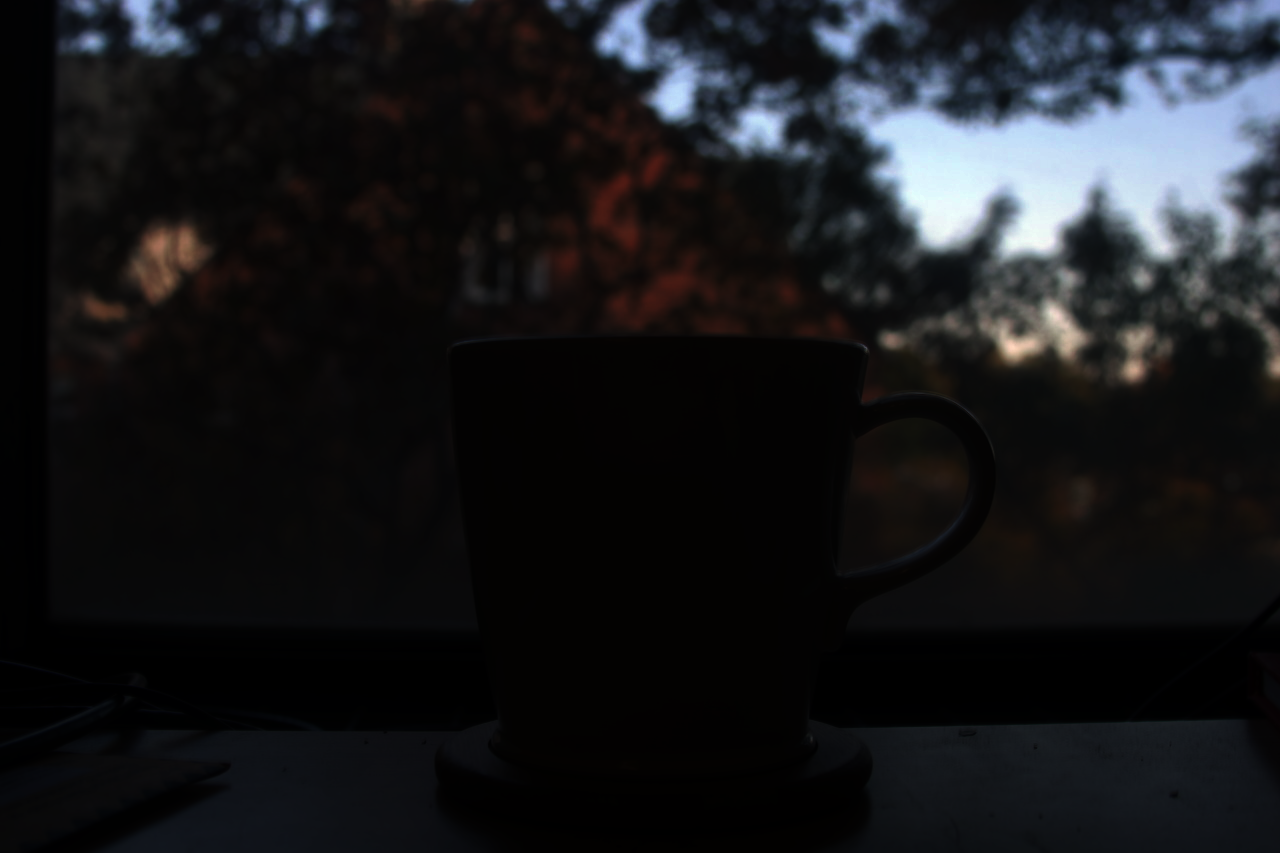
Global scale

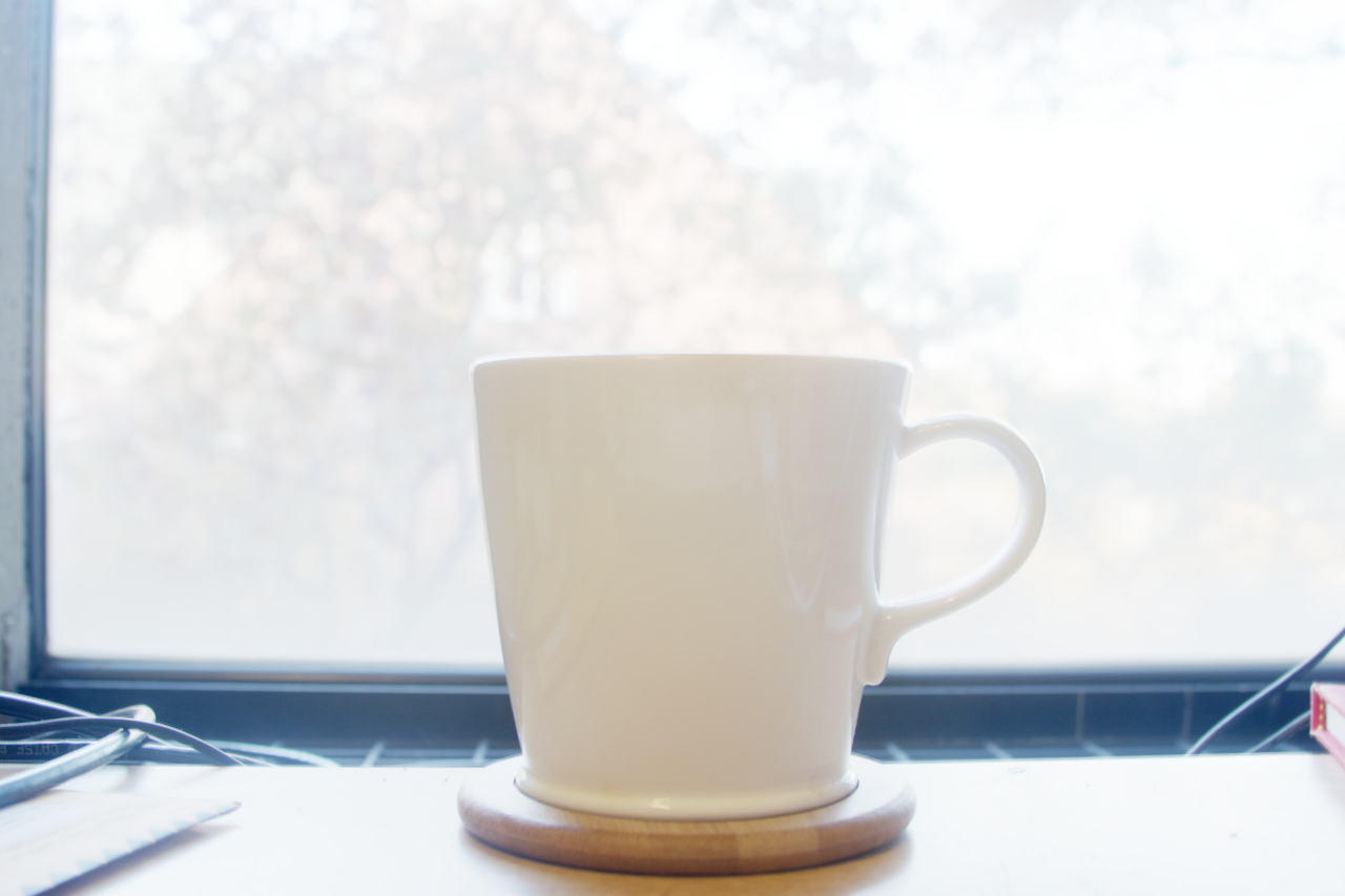
Global simple

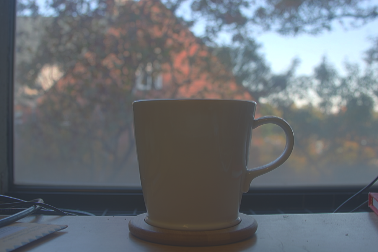
Durand

Garden

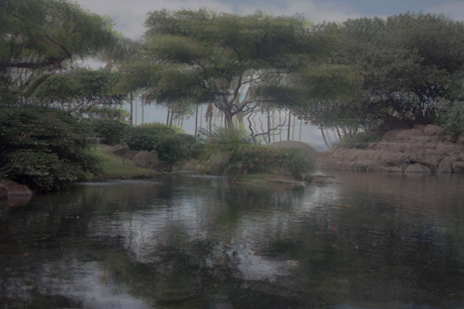
Radiance map

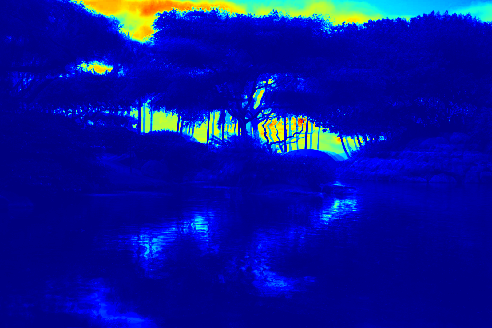
Averaged across all channels

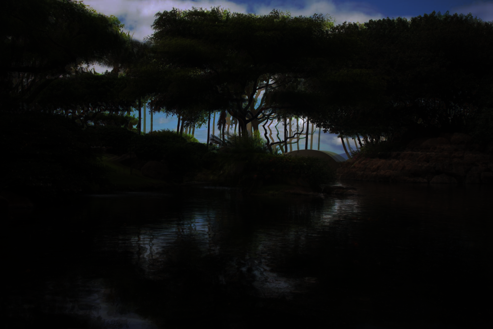
Global scale

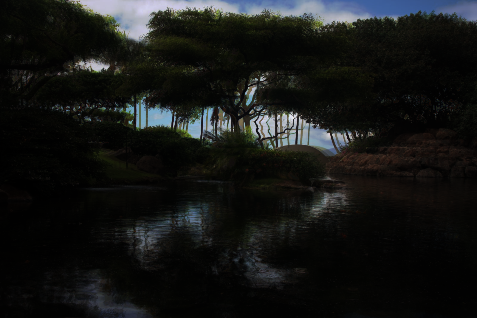
Global simple

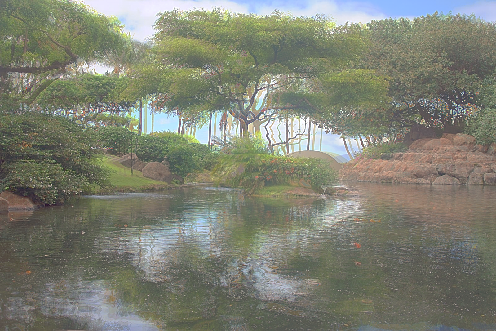
Durand

Garage

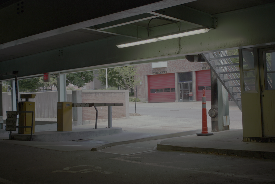
Radiance map

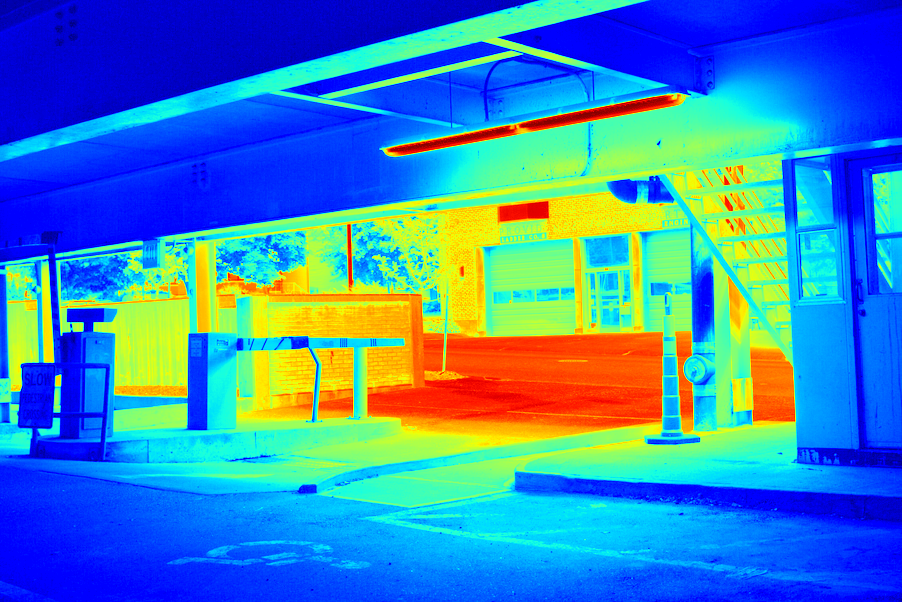
Averaged across all channels

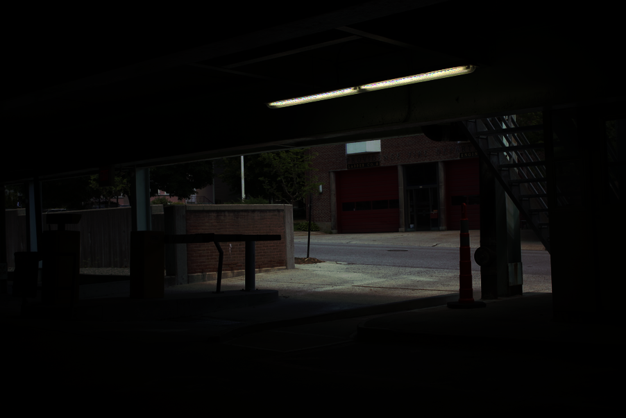
Global scale

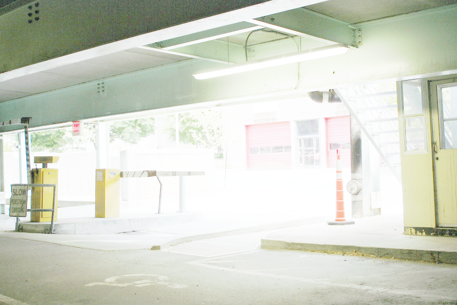
Global simple

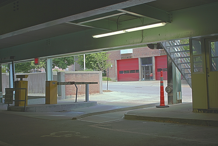
Durand

House

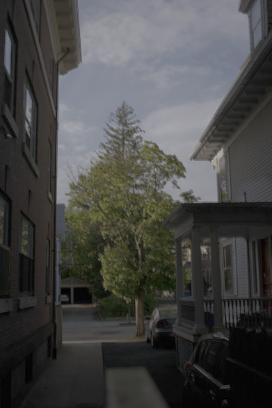
Radiance map

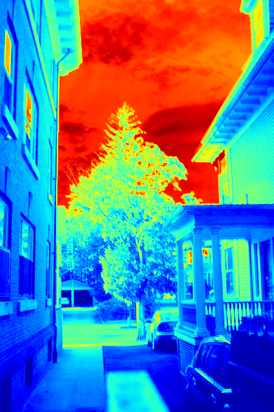
Averaged across all channels

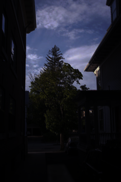
Global scale

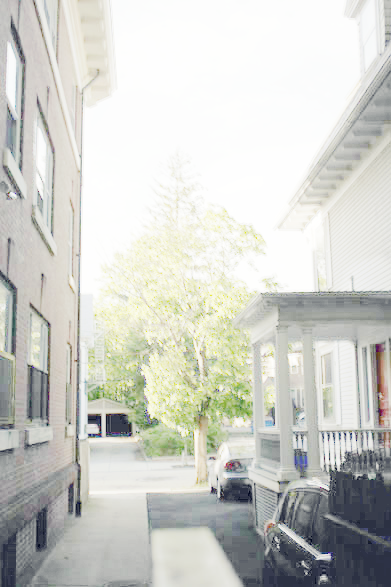
Global simple

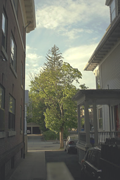
Durand

Bell & Whistle: My own images with HDR

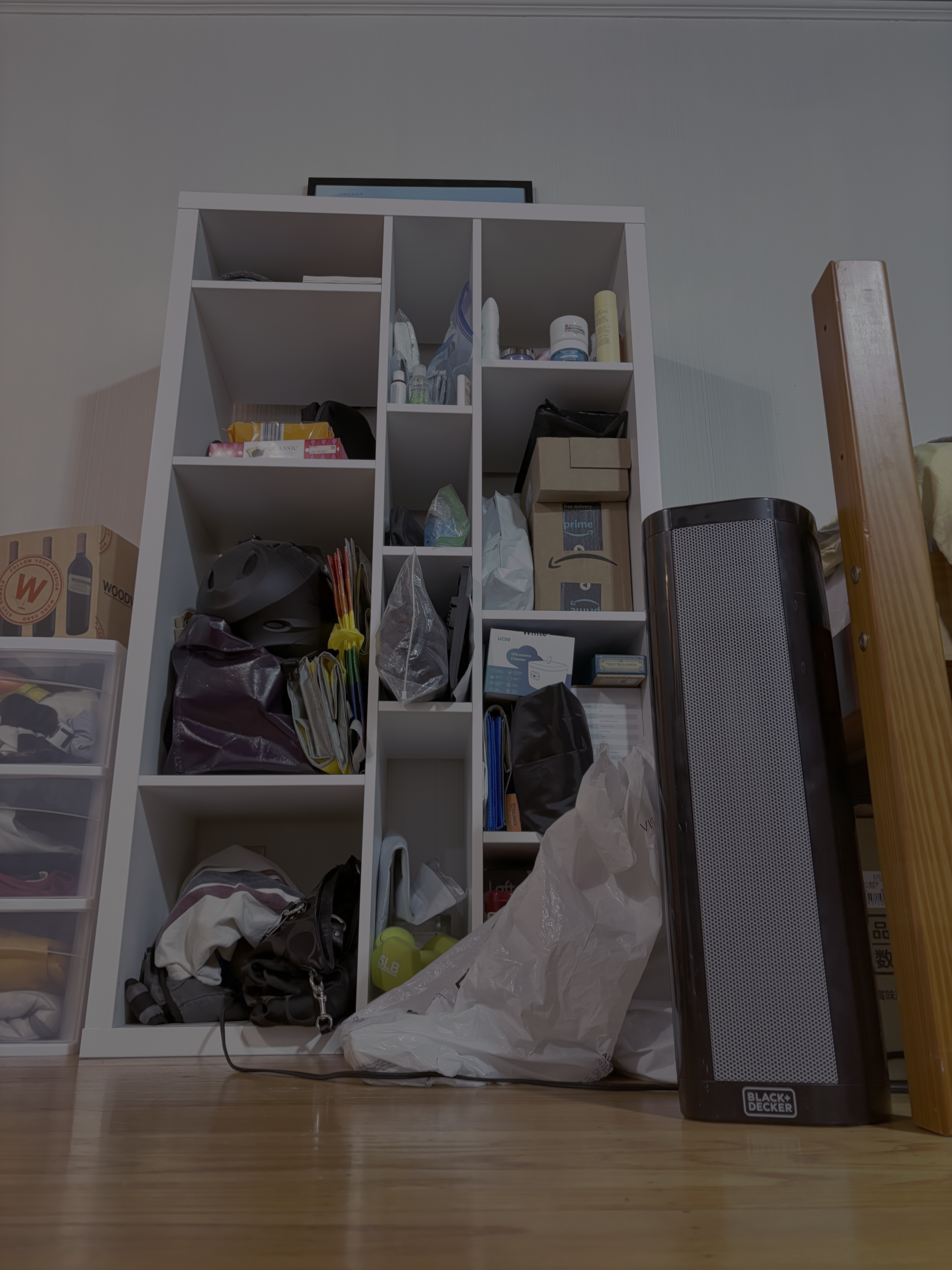
For this section I took some of my own photos using my phone. I used 4 different exposure levels per photo, and combined them using the same HDR workflow as above.

Shelf

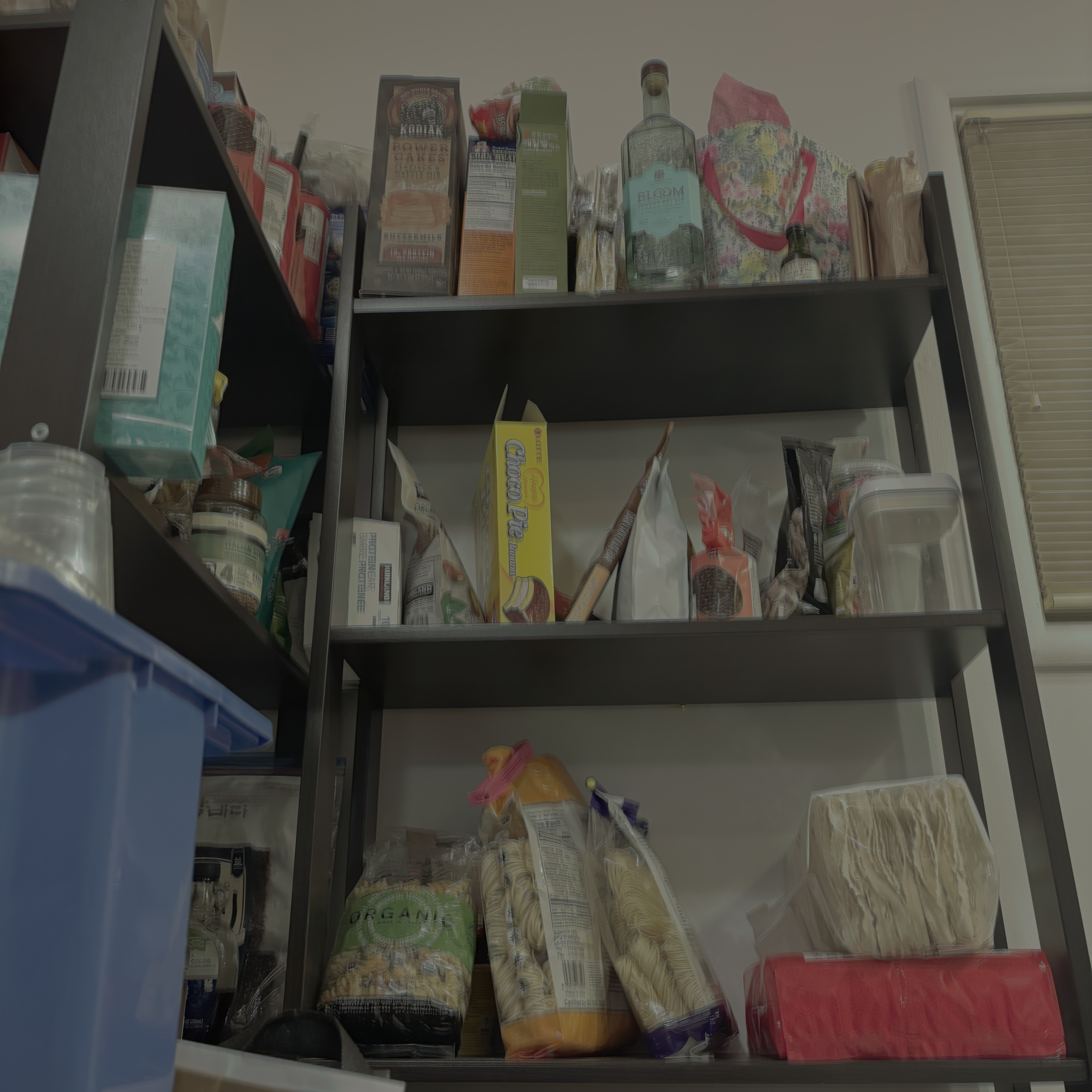
Radiance map

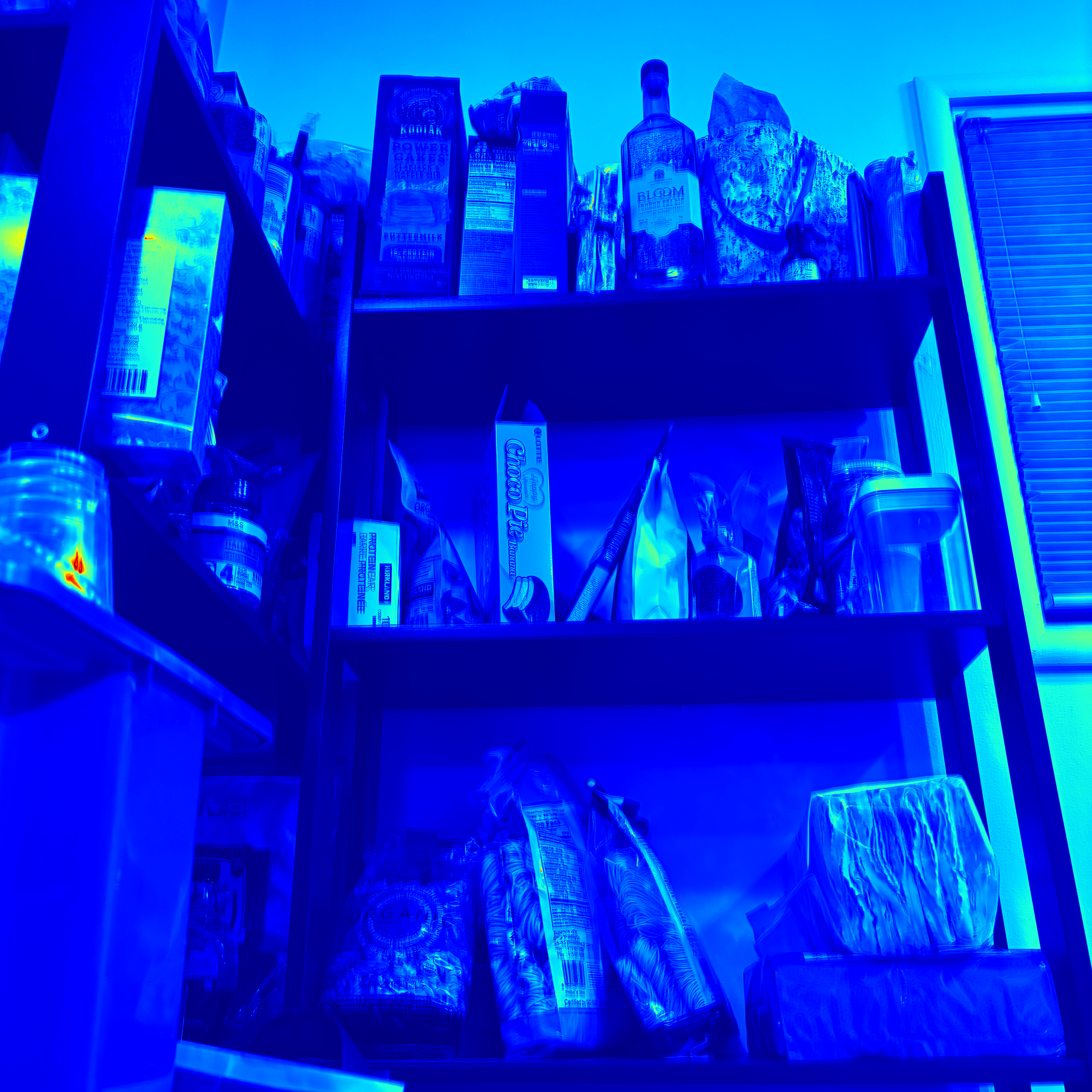
Averaged across all channels

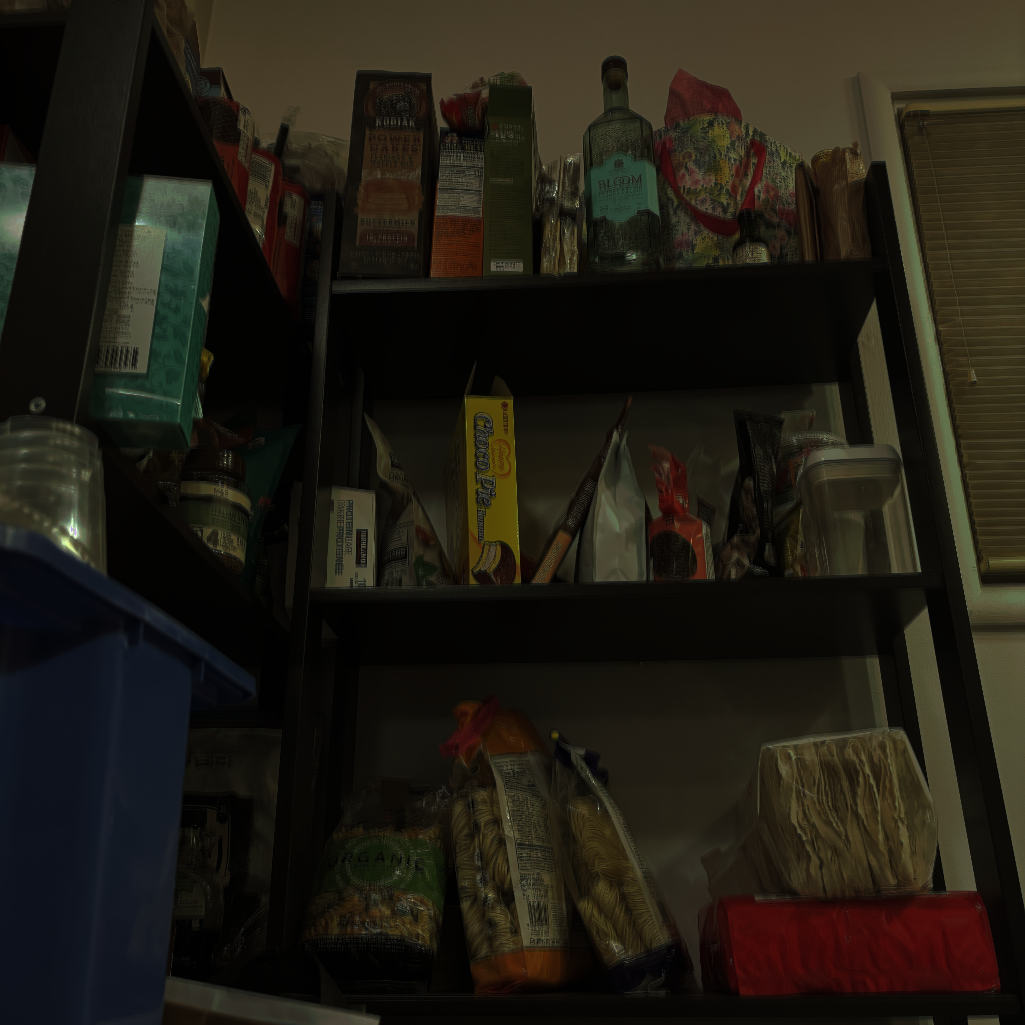
Global scale

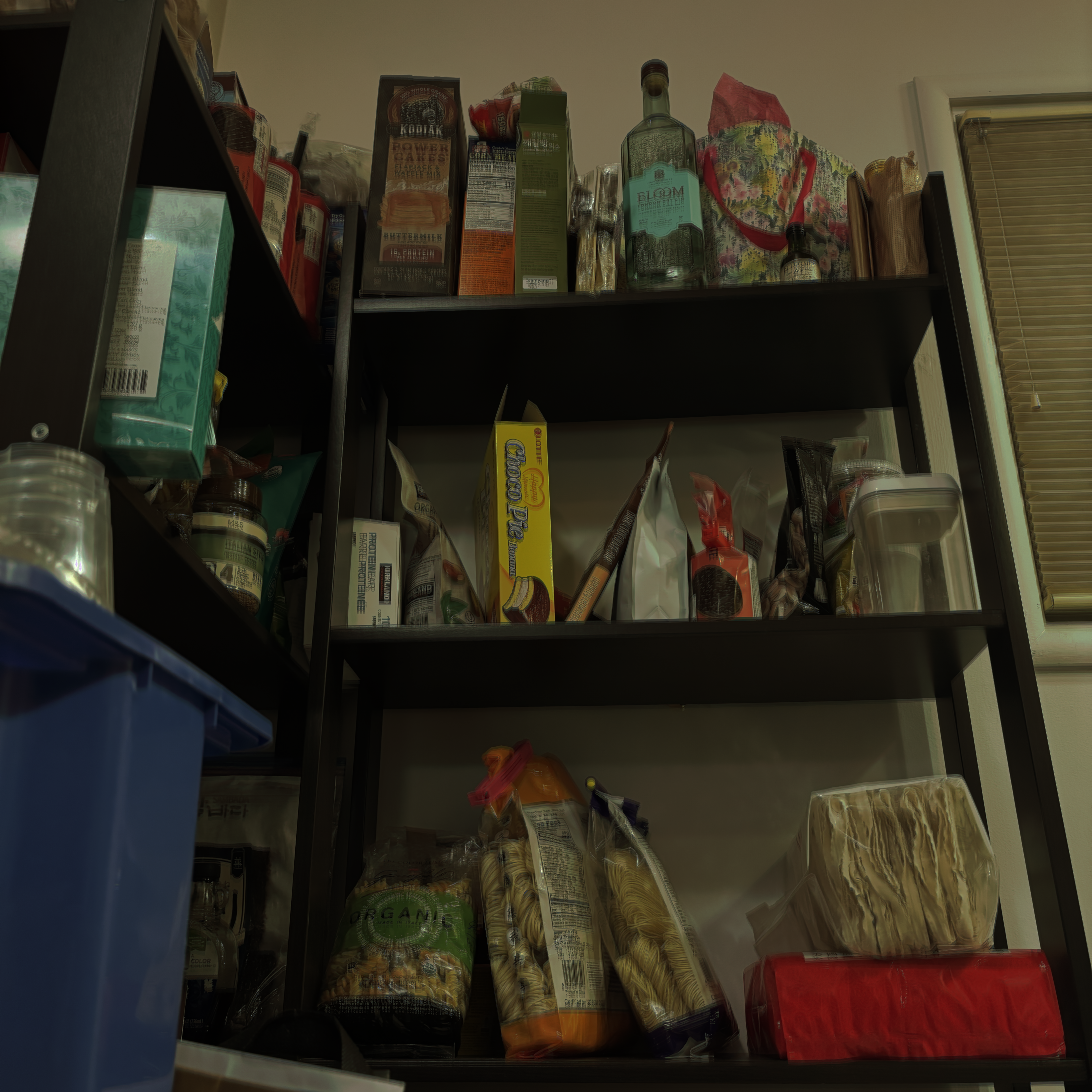
Global simple

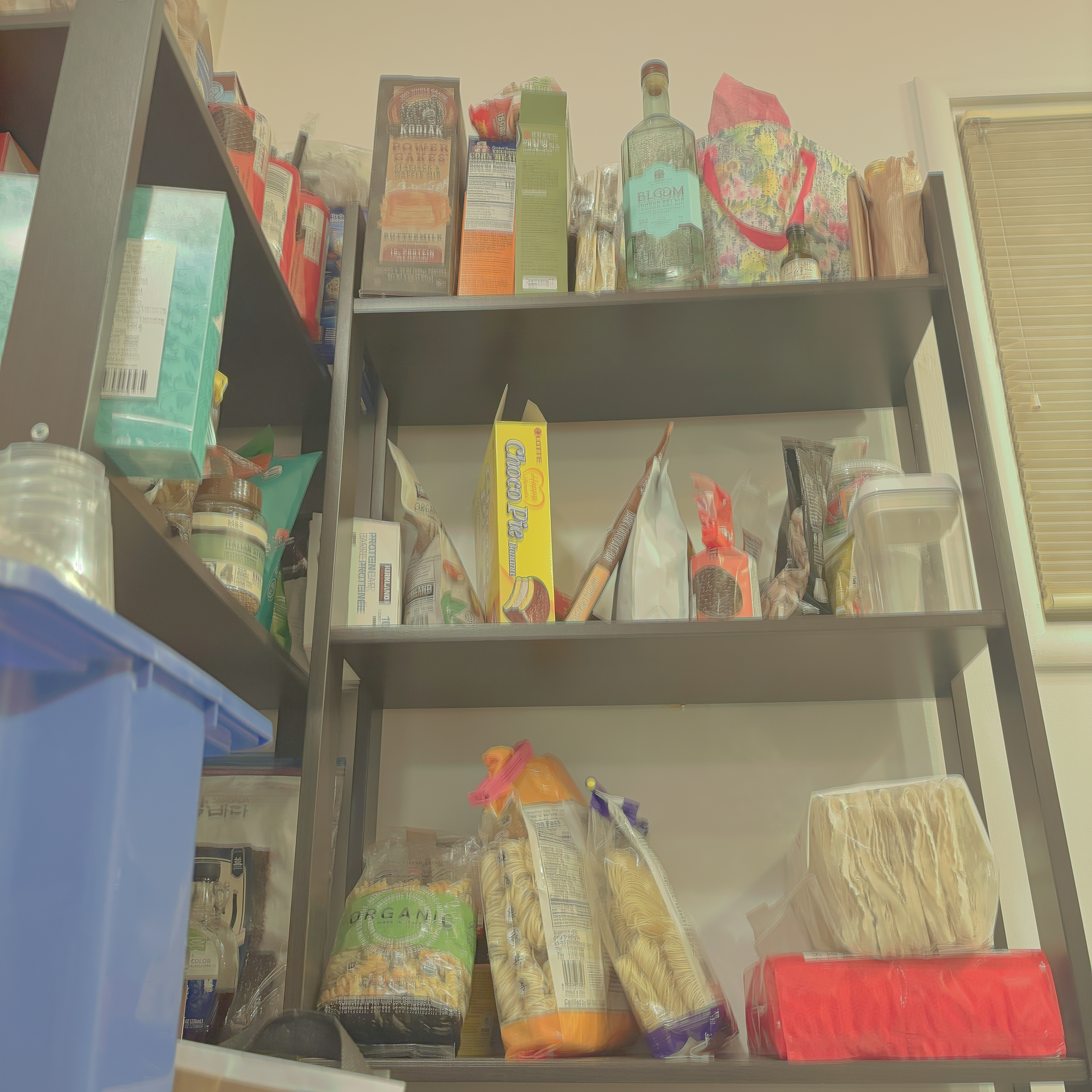
Durand

Shelf 2

Radiance map

Averaged across all channels

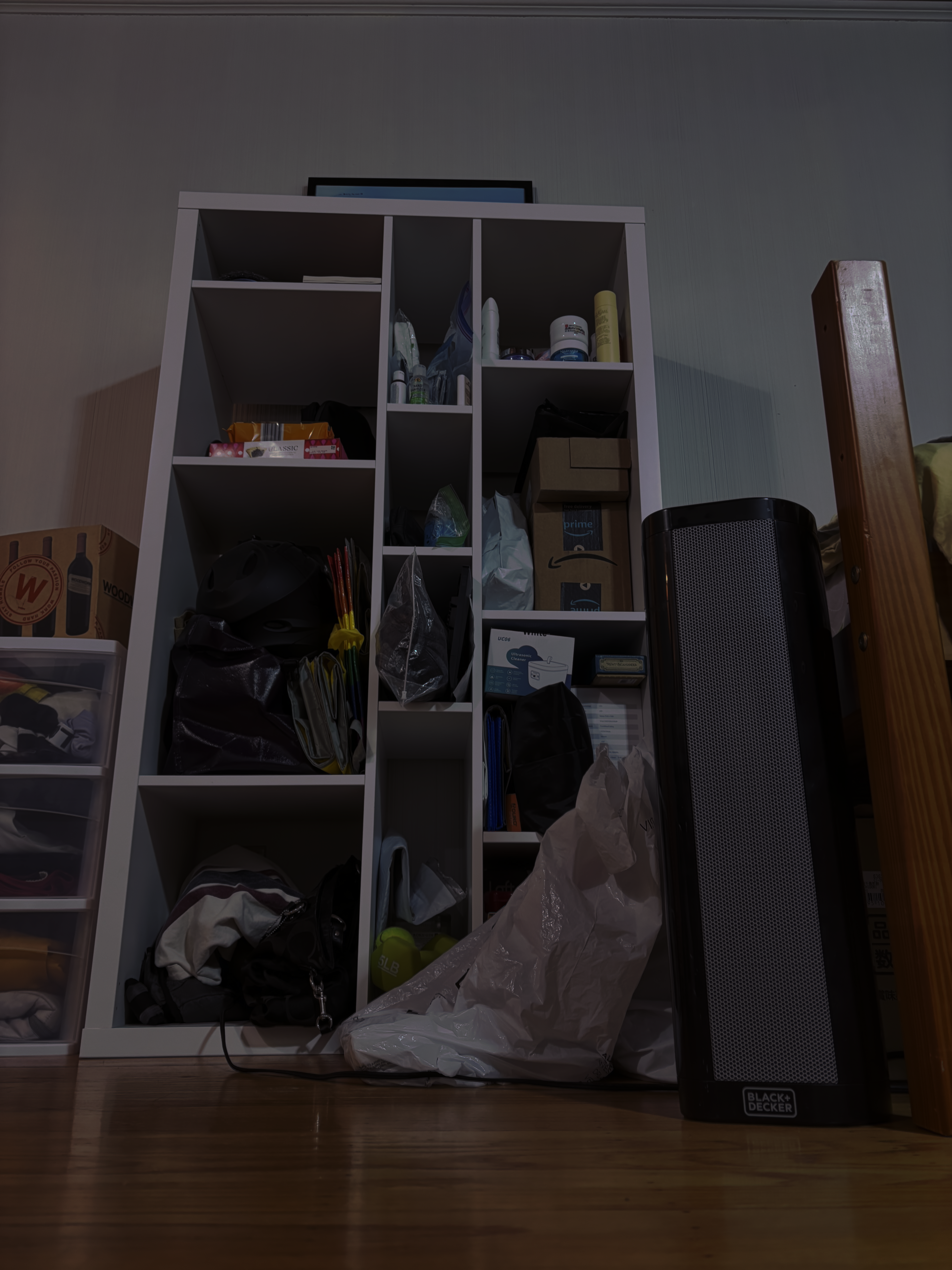
Global scale

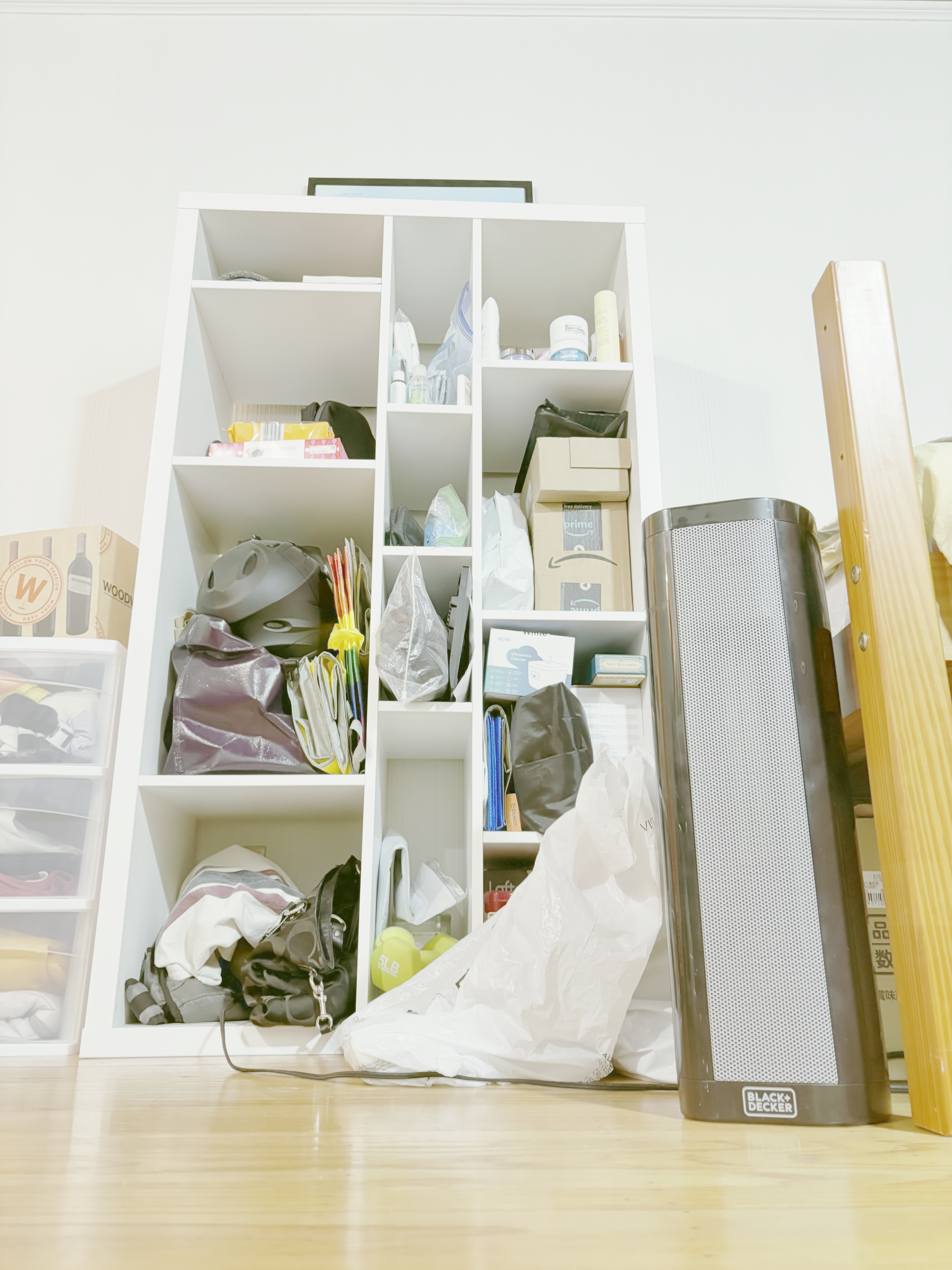
Global simple

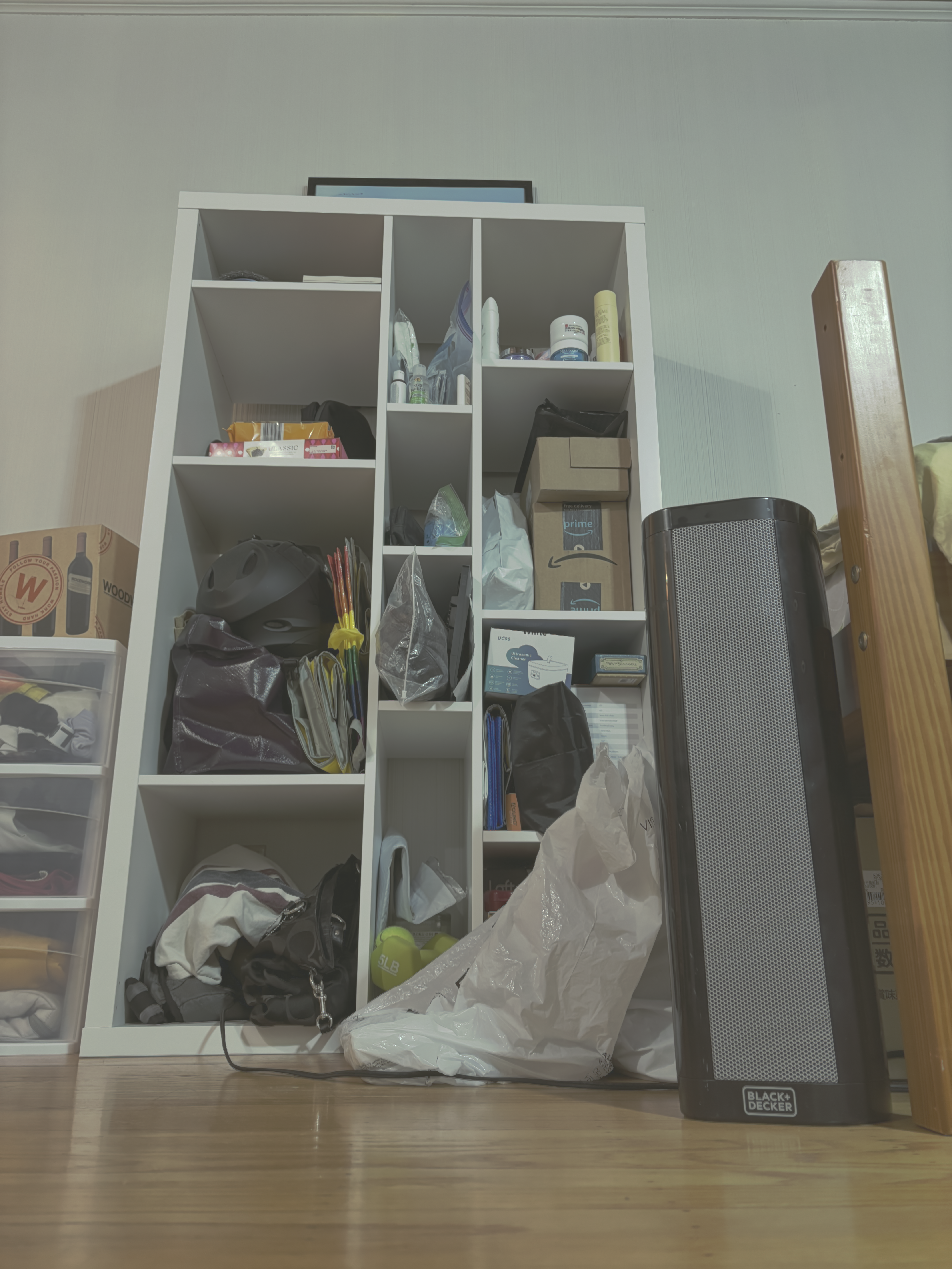
Durand

The coolest thing I have learned from this project

While initially tedious, I found the HDR project to be very satisfying and educational. I had always wondered how phones adjust for high or low exposure photos automatically using HDR, and with this project I had a chance to explore different algorithms behind the magic.